From Noise to Image: A Mathematical Reading of Diffusion Models

Diffusion models can be understood from an apparently simple idea: if we know how to destroy an image little by little until it becomes noise, perhaps we can learn the reverse path. The interesting part is that this reverse path does not consist of memorizing images or applying a classic cleaning filter. It consists of learning the local geometry of a probability distribution: where a noisy sample should move to increasingly resemble a real image.

In this article I present an implementation of diffusion models formulated through Stochastic Differential Equations (SDEs), following the framework of Song et al. ¹. The idea is not only to show generated images, but to explain why the method works, what role the score $\nabla_x \log p_t(x)$ plays, and how the reverse SDE, training via denoising score matching, samplers, and the probability flow ODE naturally arise.

The associated code is available on GitHub:

https://github.com/trentisiete/image_generation_difussion_project

---

1. The problem: learning a distribution in a huge space

An image is not just a matrix of pixels. From a probabilistic point of view, an image is a point in a very high-dimensional space. An RGB image of $32 \times 32$, like those in CIFAR-10, lives in a space of dimension $32 \cdot 32 \cdot 3 = 3072$. However, not all points in that space are natural images. Most are structureless noise. Real images occupy a very special region: they contain edges, textures, symmetries, objects, backgrounds, compatible colors, and patterns that do not appear at random.

The goal of a generative model is to approximate the distribution of real data, which we denote by $p_{\text{data}}(x)$, in order to generate new samples:

$$x \sim p_{\text{model}}(x)$$

where $p_{\text{model}}$ tries to resemble $p_{\text{data}}$.

The challenge is that $p_{\text{data}}(x)$ is not known explicitly. We have examples, but not a closed-form formula of the distribution. Diffusion models attack this problem in an elegant way: instead of trying to directly learn how to generate a clean image from scratch, they first build a process that destroys the data in a controlled manner and then learn to invert it.

---

2. The central intuition: destroying is easy, reconstructing is learning

The forward process starts with a real image $x(0) \sim p_{\text{data}}$ and gradually adds noise until obtaining a variable $x(T)$ that approximates a simple distribution, usually a Gaussian. Conceptually:

$$x(0) \longrightarrow x(t) \longrightarrow x(T) \approx \mathcal{N}(0,I)$$

This process is easy because we define it ourselves. We can choose how much noise to add and how that noise evolves over time.

The reverse process is the truly generative one:

$$x(T) \longrightarrow x(t) \longrightarrow x(0)$$

We start from pure noise and gradually remove noise until obtaining a plausible image. But here the key question arises: how does the model know where a noisy sample should move?

The answer is the score:

$$\nabla_x \log p_t(x)$$

This vector points in the direction in which the logarithmic density of the perturbed data at time $t$ increases most rapidly. Intuitively, if $x(t)$ is a noisy image, the score indicates toward which region of the space it should move to be more probable under the distribution of images with that noise level.

First important finding: the model does not need to directly learn the full distribution $p_t(x)$. It suffices to learn its gradient field. Instead of asking “what is the exact probability of this image?”, it learns “where should I move to be in a more probable region?“.

---

3. The forward process as an SDE

In continuous time, the forward diffusion process is expressed through a Stochastic Differential Equation:

$$dx = f(x,t)\,dt + g(t)\,dW(t)$$

where:

• $x(t)$ represents the sample at instant $t$.
• $f(x,t)$ is the drift term, which introduces a deterministic evolution.
• $g(t)$ controls the intensity of the noise.
• $W(t)$ is a standard Wiener process, i.e., Brownian motion.

The SDE combines two effects. The term $f(x,t)\,dt$ pushes the sample deterministically, while $g(t)\,dW(t)$ introduces randomness. In the diffusion context, that randomness is precisely the mechanism that transforms structured data into noise.

3.1. Variance Exploding SDE

The VE-SDE is defined as:

$$dx = \sqrt{\frac{d[\sigma^2(t)]}{dt}}\,dW(t)$$

Here there is no deterministic drift, since $f(x,t)=0$. The data retains its center, but its variance increases over time. That is why it is called Variance Exploding: the variance grows progressively until the original signal is dominated by noise.

The transition of the forward process has Gaussian form:

$$p_{0t}(x(t)\mid x(0)) = \mathcal{N}\left(x(t);\,x(0),\, [\sigma^2(t)-\sigma^2(0)]I\right)$$

In this family, the data is perturbed by adding increasingly intense noise around the original image.

3.2. Variance Preserving SDE

The VP-SDE has the form:

$$dx = -\frac{1}{2}\beta(t)x(t)\,dt + \sqrt{\beta(t)}\,dW(t)$$

Unlike the VE-SDE, here there is drift. The term

$$-\frac{1}{2}\beta(t)x(t)$$

progressively contracts the signal, while the stochastic term adds noise. The combination is designed to preserve the overall variance when the data is normalized.

Its transition is also Gaussian:

$$p_{0t}(x(t)\mid x(0)) = \mathcal{N}\left( x(t); x(0)e^{-\frac{1}{2}\int_0^t \beta(s)\,ds}, \left[1-e^{-\int_0^t \beta(s)\,ds}\right]I \right)$$

This equation is very revealing: the mean of the image fades away with the exponential factor, while the variance of the noise increases in a complementary manner. The signal does not disappear all at once; it dissolves following a controlled trajectory.

3.3. Sub-VP SDE

The sub-VP SDE modifies the diffusion term:

$$dx = -\frac{1}{2}\beta(t)x(t)\,dt + \sqrt{\beta(t)\left(1-e^{-2\int_0^t \beta(s)\,ds}\right)}\,dW(t)$$

This variant maintains a structure similar to the VP-SDE, but adjusts the amount of noise introduced at each instant. In practice it can produce better results in terms of likelihood, although it does not always necessarily match the best perceptual quality.

---

4. The mathematical turn: inverting a diffusion

Up to this point we have only defined how to destroy an image. The generative part appears when we use Anderson’s result on time-reversed diffusion processes ². If the forward process is:

$$dx = f(x,t)\,dt + g(t)\,dW(t)$$

then there exists a reverse process that allows traversing the same marginal distributions in the opposite direction:

$$dx = \left[ f(x,t) - g(t)^2 \nabla_x \log p_t(x) \right]dt + g(t)\,d\bar{W}(t)$$

where $d\bar{W}(t)$ represents Brownian motion in reverse time.

This equation contains the core of score-based diffusion models. Everything known about the forward process appears in $f$ and $g$. What is unknown is concentrated in a single term:

$$\nabla_x \log p_t(x)$$

That is, to invert the diffusion we do not need to learn the entire dynamics from scratch. We need to estimate the score of the perturbed distribution at each instant.

Second important finding: generation reduces to learning a vector field. If the model knows how to estimate, at each noise level, where the density of images increases, it can guide a sample from noise to a region where realistic images live.

In practice, a neural network $s_\theta(x,t)$ is trained to approximate:

$$s_\theta(x,t) \approx \nabla_x \log p_t(x)$$

Substituting the real score with the learned score, the reverse SDE becomes:

$$dx = \left[ f(x,t) - g(t)^2 s_\theta(x,t) \right]dt + g(t)\,d\bar{W}(t)$$

This is the equation that is discretized during sampling.

---

5. How the score is trained without knowing the density

At first glance it seems we have a circular problem. We want to train a network to approximate $\nabla_x \log p_t(x)$, but we do not know $p_t(x)$. If we do not know the distribution, how do we obtain the training label?

The key lies in not directly using the unknown marginal score, but rather the conditional score of the perturbation process, which we do know because we defined the forward process ourselves.

For many SDEs used in diffusion, the forward transition can be written as a Gaussian:

$$p_{0t}(x(t)\mid x(0)) = \mathcal{N}\left(x(t);\mu_t(x(0)),\sigma_t^2 I\right)$$

where $\mu_t(x(0))$ is the mean at time $t$ and $\sigma_t^2$ the variance of the added noise.

Now we compute the score of this Gaussian with respect to $x(t)$. The logarithmic density, ignoring constants that do not depend on $x(t)$, is:

$$\log p_{0t}(x(t)\mid x(0)) = -\frac{1}{2\sigma_t^2} \left\|x(t)-\mu_t(x(0))\right\|_2^2 + C$$

Differentiating with respect to $x(t)$:

$$\nabla_{x(t)} \log p_{0t}(x(t)\mid x(0)) = -\frac{x(t)-\mu_t(x(0))}{\sigma_t^2}$$

This equation is one of the most elegant points of the method. If we generate a noisy sample $x(t)$ from a clean image $x(0)$, we know exactly what the conditional score should be that points back toward the mean of the perturbation.

Third important finding: the noise-adding process itself generates the training labels. We do not need to annotate images, nor know $p_{\text{data}}(x)$, nor compute an intractable density. It suffices to take an image, perturb it, and teach the network to predict the vector that undoes that perturbation.

The denoising score matching loss function in continuous time is:

$$\theta^* = \arg\min_\theta \mathbb{E}_{t \sim \mathcal{U}(0,T)} \left[ \lambda(t) \mathbb{E}_{x(0)\sim p_{\text{data}}} \mathbb{E}_{x(t)\mid x(0)} \left[ \left\| s_\theta(x(t),t) - \nabla_{x(t)} \log p_{0t}(x(t)\mid x(0)) \right\|_2^2 \right] \right]$$

Substituting the Gaussian conditional score:

$$\left\| s_\theta(x(t),t) + \frac{x(t)-\mu_t(x(0))}{\sigma_t^2} \right\|_2^2$$

The network learns, for each noise level, how a perturbed sample must be corrected to move back toward a high-probability zone.

---

6. From score to sampling: how an image appears

Once $s_\theta(x,t)$ is trained, generation consists of numerically solving the reverse SDE from $t=T$ to $t=0$. It is initialized as:

$$x(T) \sim p_T(x)$$

usually a Gaussian, and a reverse-time integrator is applied.

6.1. Euler-Maruyama

Euler-Maruyama is the basic integrator for SDEs. If we discretize time as $t_N=T,\dots,t_0=0$, a reverse step can be interpreted as:

$$x_{i-1} = x_i + \left[ f(x_i,t_i) - g(t_i)^2 s_\theta(x_i,t_i) \right]\Delta t + g(t_i)\sqrt{|\Delta t|}\,z_i$$

with:

$$z_i \sim \mathcal{N}(0,I)$$

This method combines a deterministic correction, guided by the score, with a random term that maintains the stochastic nature of the process.

6.2. Predictor-Corrector

Predictor-Corrector samplers add a second idea. The predictor moves forward in reverse time, for example with Euler-Maruyama. The corrector, on the other hand, refines the sample at the same noise level through steps inspired by Langevin dynamics.

The corrector can be seen as a way of saying: “before moving to the next noise level, let’s adjust the sample a bit more so that it is more probable under $p_t$”. This tends to improve visual quality, because it not only advances toward less noise, but also corrects the position within each intermediate distribution.

6.3. Probability Flow ODE

The SDE framework has a particularly interesting property: there exists a deterministic ODE whose trajectories share the same marginal distributions as the SDE. This probability flow ODE is written as:

$$dx = \left[ f(x,t) - \frac{1}{2}g(t)^2\nabla_x \log p_t(x) \right]dt$$

Substituting the real score with the learned one:

$$dx = \left[ f(x,t) - \frac{1}{2}g(t)^2s_\theta(x,t) \right]dt$$

Fourth important finding: the same score model allows two forms of generation. One stochastic, through the reverse SDE, and another deterministic, through the probability flow ODE. The first preserves noise during sampling; the second transforms an initial condition into a unique trajectory.

The ODE also allows estimating likelihoods through the instantaneous change of variables formula ³. If $p_t(x(t))$ evolves following an ODE $dx/dt = v_t(x)$, then:

$$\frac{d \log p_t(x(t))}{dt} = -\nabla_x \cdot v_t(x(t))$$

In SDE-based diffusion, this allows computing metrics such as NLL or Bits Per Dimension (BPD), something not all generative models offer naturally.

---

7. Conditional generation: steering the process toward a class

Unconditional generation produces images without specifying a category. To condition the process on a class $y$, an auxiliary time-dependent classifier $p_\phi(y\mid x(t),t)$ can be used.

The derivation starts from Bayes:

$$p_t(x\mid y) = \frac{p_t(y\mid x)p_t(x)}{p_t(y)}$$

We take logarithms:

$$\log p_t(x\mid y) = \log p_t(y\mid x) + \log p_t(x) - \log p_t(y)$$

We differentiate with respect to $x$:

$$\nabla_x \log p_t(x\mid y) = \nabla_x \log p_t(x) + \nabla_x \log p_t(y\mid x)$$

because $p_t(y)$ does not depend on $x$.

This equation has a very clear interpretation: the conditional score is the unconditional score plus an additional force that pushes the image toward the desired class.

In the implementation it is approximated as:

$$\nabla_x \log p_t(x\mid y) \approx s_\theta(x,t) + w \nabla_x \log p_\phi(y\mid x,t)$$

where $w$ controls the intensity of the guidance. Thus, the conditional reverse SDE becomes:

$$dx = \left[ f(x,t) - g(t)^2 \left( s_\theta(x,t) + w\nabla_x \log p_\phi(y\mid x,t) \right) \right]dt + g(t)d\bar{W}(t)$$

In practical terms, the score model contributes general knowledge about what images look like, while the classifier introduces a semantic preference: “I want this image to end up resembling a plane, a dog, a ship, or a frog”.

---

8. Imputation: generating only what’s missing

The same idea can also be used to impute hidden regions of an image. Let $m$ be a binary mask, where $m=1$ indicates known pixels and $m=0$ indicates areas to be reconstructed.

During reverse sampling, the model proposes a complete image. However, at each step the known part is replaced by a perturbed version of the original image at the same noise level. The update can be expressed as:

$$x'_{t_{i-1}} = m \odot \tilde{x}_{t_{i-1}} + (1-m)\odot x_{t_{i-1}}$$

where:

• $\tilde{x}_{t_{i-1}}$ is the original image perturbed through the forward process up to instant $t_{i-1}$.
• $x_{t_{i-1}}$ is the sample generated by the model.
• $\odot$ denotes element-wise product.

The interpretation is simple: the model is free to invent the unknown regions, but must respect the observed information. This strategy turns an unconditional generative model into a context-conditioned reconstruction tool.

---

9. Implementation: theory translated into components

The implementation was organized so that each mathematical concept had a direct representation in code. SDEs were implemented as objects capable of providing their drift and diffusion coefficients, their transition distributions, and the operations needed to train the score.

The main elements were:

• SDE families: VE-SDE, VP-SDE, and Sub-VP SDE.
• Linear and cosine noise schedules.
• U-Net-based score models.
• Samplers: Euler-Maruyama, Predictor-Corrector, Probability Flow ODE, and exponential integrators.
• Metrics: FID, Inception Score, NLL, and BPD.
• Extensions for conditional generation and imputation.

The U-Net architecture is especially well suited because it combines local and global information. In images, small structures —edges, textures, contours— must coexist with larger-scale relationships, such as shape, object, and background. Skip connections allow spatial detail to be recovered while deeper layers capture context.

---

10. Results: what is observed when generating images

Experimentation was carried out mainly with CIFAR-10 and MNIST. To illustrate the system’s behavior, representative results are shown using a linear VP-SDE and different sampling methods.

The sequence visually shows the central idea of the method: generation does not appear all at once. First color masses form, then textures, later recognizable structures, and finally more defined details. This behavior fits the probabilistic interpretation: at first, very noisy and smooth distributions are resolved; toward the end, work happens at low noise levels, where fine details matter.

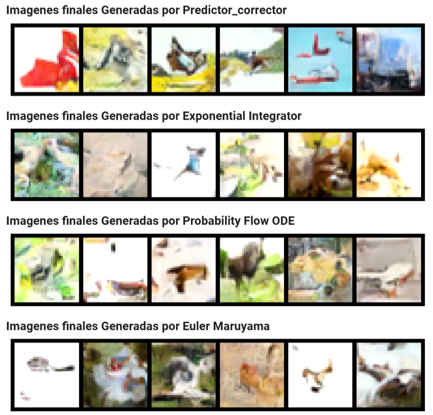
In the comparisons, Predictor-Corrector tends to produce visually more stable results, because it combines temporal advancement and local refinement. Euler-Maruyama is simpler, but usually requires more steps. The Probability Flow ODE offers a deterministic trajectory and is especially relevant when likelihood estimation is of interest.

---

11. Metrics: FID, IS, and BPD don’t tell the same story

Quantitative evaluation was carried out with metrics common in generative models: Fréchet Inception Distance (FID), Inception Score (IS), and Bits Per Dimension (BPD).

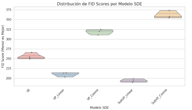
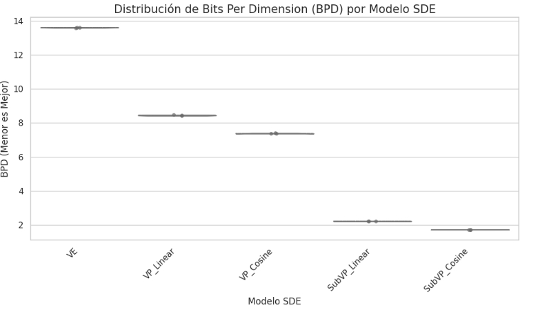
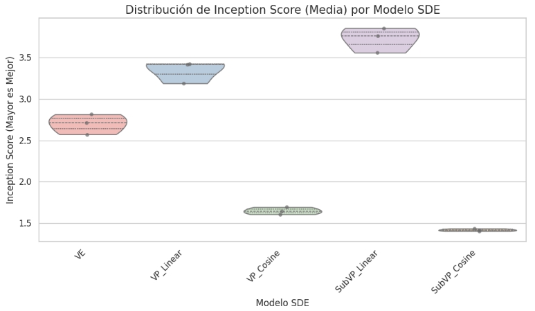
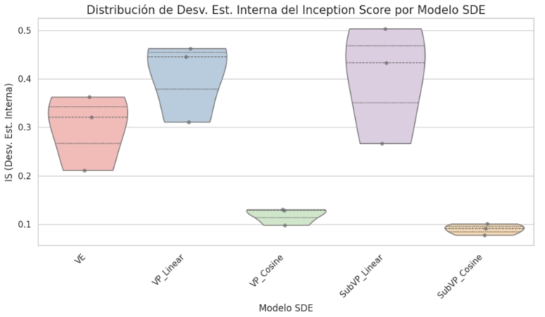
The results show an important point: not all metrics reward the same thing. In the runs performed, linear SubVP-SDE obtained the best relative perceptual results, with lower FID and higher IS. In contrast, the cosine-schedule variants stood out in BPD, especially cosine SubVP-SDE.

This difference is relevant because BPD measures probabilistic fit, while FID and IS are closer to perceptual quality and semantic diversity. A model can assign good probability to the data and still not produce the most visually convincing samples. This decoupling between likelihood and perceptual quality is one of the most important lessons when evaluating generative models.

Fifth important finding: the “best” model depends on what “best” means. If we’re looking for visually convincing images, FID and IS may be more informative. If we’re looking for probabilistic modeling and likelihood, BPD offers a different reading. Evaluation must look at several metrics, not just one.

---

12. Conditional generation

For conditional generation, a time-dependent classifier was used, based on a Wide ResNet-type architecture, trained to recognize classes even when the image is perturbed by noise.

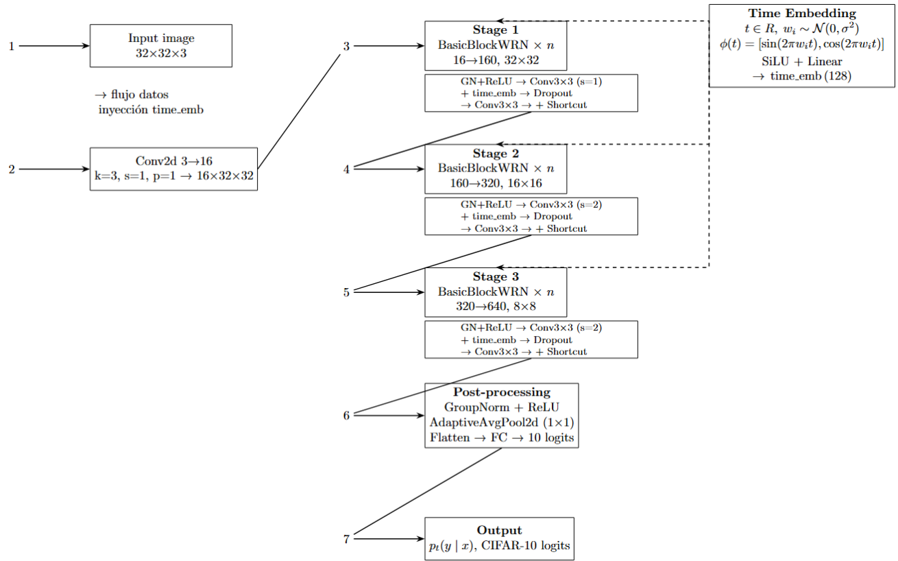
The classifier provides the term $\nabla_x \log p_\phi(y\mid x,t)$, which modifies the effective score during sampling. In this way, generation stops being completely free and is oriented toward a specific class.

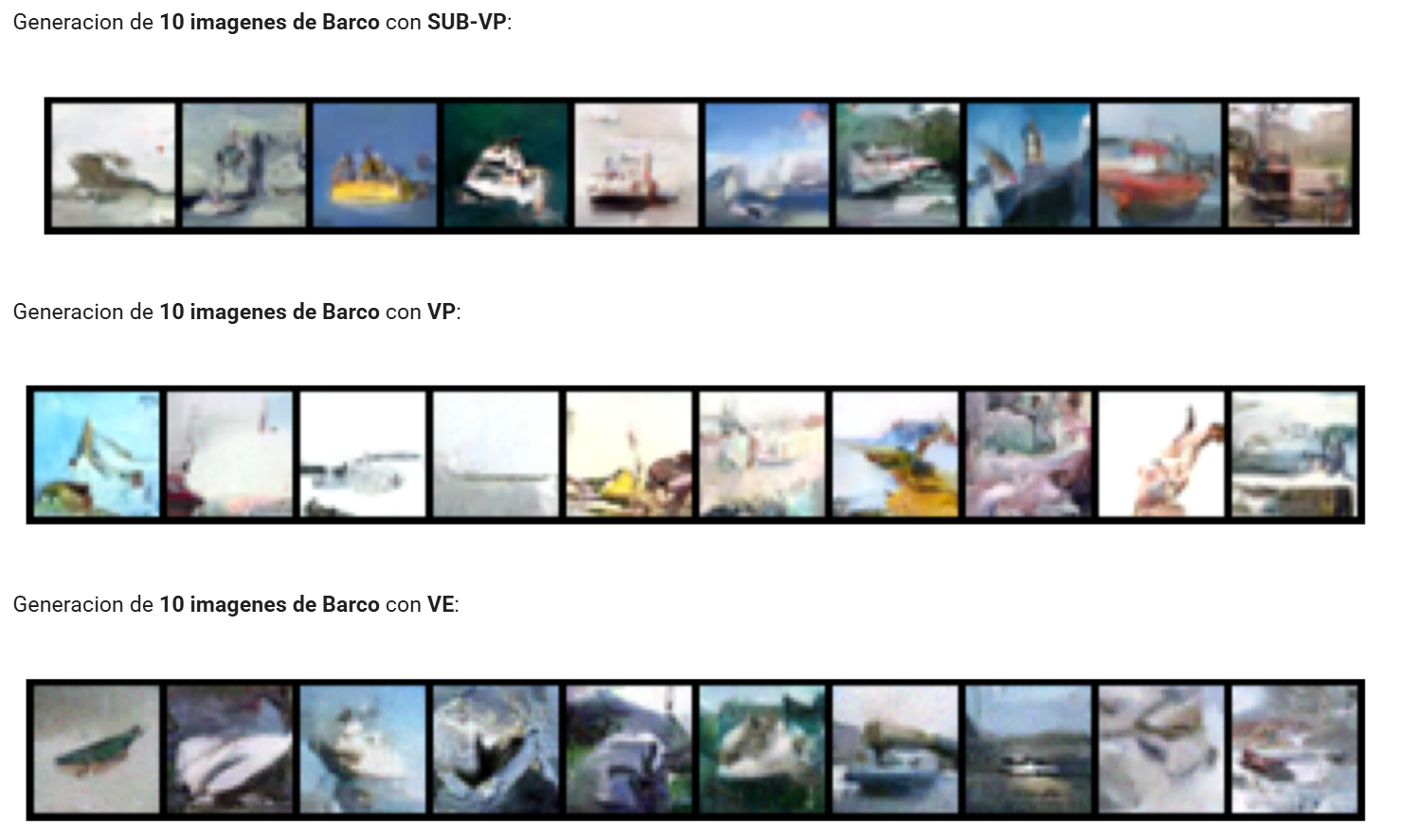
Conditional generation showed that the SDE framework serves not only to produce random images, but also to partially control the outcome. The degree of control depends on the classifier, the guidance scale, and the quality of the score model. A scale that is too low may not sufficiently steer the sample; a scale that is too high can force artifacts or reduce diversity.

---

13. Image imputation

In the imputation task, masks derived from MNIST digits were applied to CIFAR-10 images. The model had to reconstruct the hidden regions while maintaining coherence with the visible context.

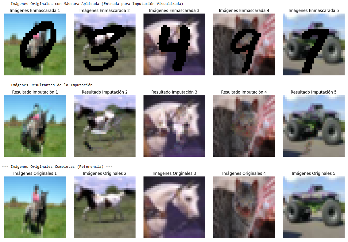
Imputation is interesting because it demonstrates that the model does not only generate from pure noise. It can also act as a prior distribution over natural images: when information is missing, it proposes content compatible with what is observed. In other words, the model does not “recover” the exact lost region, but generates a plausible reconstruction under the learned distribution.

---

14. Convergence during training

The evolution of the loss during the first 50 epochs was also compared for different SDE configurations.

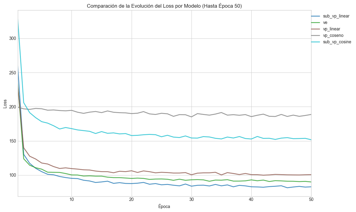
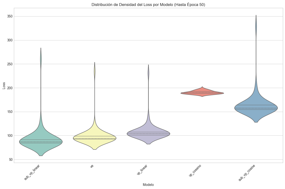
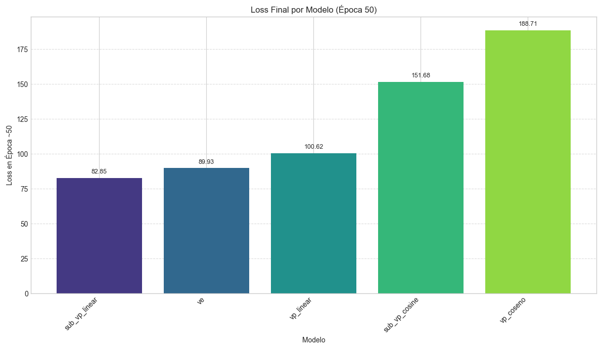
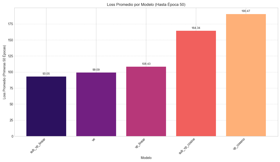
The curves suggest that linear SubVP-SDE and VE-SDE reach low loss values earlier. However, this reading should be interpreted with caution: minimizing the training loss better does not automatically guarantee better images. The loss measures the accuracy of the score estimation under the chosen perturbation scheme, while generative quality also depends on the sampler, the noise schedule, the architecture, and how errors propagate during reverse integration.

---

15. Limitations

The project has limitations that should be made explicit. Training the score models and the time-dependent classifiers is computationally costly, which restricted the number of epochs and the thoroughness of some comparisons. The evaluation of metrics such as FID was carried out on subsets of data, so the absolute values could vary. Added to this is the inherent volatility of generative model evaluation metrics: no single metric on its own captures all the desirable aspects of generation.

---

16. Conclusion: what the SDE framework makes clear

The SDE formulation offers an especially clear way to understand diffusion models. The forward process turns data into noise through a known dynamic. The reverse process allows data to be generated, but requires knowing the score of the intermediate distributions. Since that score is not available, it is approximated with a neural network trained via denoising score matching.

The most powerful aspect of the approach is that many pieces fit together naturally:

• The forward SDE defines how the data is corrupted.
• The score indicates how to move back toward regions of high probability.
• The reverse SDE transforms noise into images.
• The Probability Flow ODE offers a deterministic alternative and allows likelihood estimation.
• Classifier guidance enables conditional generation.
• Imputation emerges by combining reverse sampling with constraints on known pixels.

From an experimental standpoint, the results show that there is no single universally superior configuration. Linear SubVP-SDE performed better on perceptual metrics such as FID and IS, while cosine variants stood out in BPD. This difference reinforces an important idea: evaluating generative models requires looking simultaneously at visual quality, diversity, stability, computational cost, and probabilistic fit.

Taken together, this work made it possible to connect theory, implementation, and experimentation within a single framework: from the mathematical derivation of the score to image generation, conditional generation, and imputation.

---

References

Footnotes

1. Song, Y., Sohl-Dickstein, J., Kingma, D. P., Kumar, A., Ermon, S., & Poole, B. (2021). Score-Based Generative Modeling through Stochastic Differential Equations. In International Conference on Learning Representations (ICLR). ↩

2. Anderson, B. D. (1982). Reverse-time diffusion equation models. Stochastic Processes and their Applications, 13(3), 313-326. ↩

3. Chen, R. T., Rubanova, Y., Bettencourt, J., & Duvenaud, D. K. (2018). Neural ordinary differential equations. In Advances in neural information processing systems (NeurIPS). ↩