Surrogate models for finding optimal inputs

This article compiles my Bachelor’s Thesis in Data Science and Engineering. It studies how to use Gaussian processes as surrogate models to learn from few evaluations, quantify uncertainty, and decide which configurations are worth trying next.

The code, experiments, and reproduction materials are available on GitHub:

https://github.com/trentisiete/surrogate_models

---

Abstract

In numerous experimental contexts, the main difficulty lies not only in analyzing the results obtained, but in deciding which experiments to carry out next when each evaluation entails a high cost. In this context, the UAM’s Healthy Food Ingredients Group presented us with a problem oriented toward optimizing the selection of new experimental configurations in feeding Hermetia illucens larvae.

The ideal tool for these problems is surrogate models, which consist of building a machine learning model that approximates the relationship between the characteristics of a diet and the results one would expect from it. In this way, before carrying out a new trial, the model can help estimate which food combinations seem most promising and with what degree of confidence such predictions are made. In particular, the surrogate models will be based on Gaussian processes, since they allow combining prediction and uncertainty within the same framework.

The thesis is developed in three stages. First, the theoretical framework necessary to understand surrogate models, Gaussian processes, and how uncertainty can be used to propose new evaluations is established. Second, synthetic experiments are carried out on known functions, which allows the behavior of these tools to be studied in a controlled way: starting from few initial data points, fitting a model, selecting new points via Expected Improvement, and checking whether the process improves the best result found so far. These experiments show that the proposed procedure improves the initial design in all the benchmarks analyzed, although its performance depends on various factors.

Finally, the methodology is applied to the real case of diets for Hermetia illucens. In this scenario, the model is evaluated by leaving out complete diets during training and checking whether it is able to predict their results. This form of evaluation was chosen because it approximates the real intended use: estimating the behavior of a diet not yet tested and choosing the model that best generalizes to new proposals. The results indicate that, in the three objectives finally analyzed, the Gaussian process improves on the baseline model, although the predictive uncertainty appears only partially calibrated.

Taken together, the work shows that surrogate models do not replace experimental validation, but they can reduce the search space, quantify uncertainty, and prioritize new candidate configurations when the experimental budget is limited.

Introduction

Many real optimization problems consist of finding an input configuration that produces a favorable response. However, in numerous engineering, data science, or physical experimentation contexts, evaluating each configuration can be costly, slow, or limited. In these cases, it is not feasible to exhaustively explore the entire search space or directly apply methods that require many evaluations of the objective function. The problem is no longer only finding the best point, but rather deciding how to learn as much as possible from a reduced number of observations.

This scenario arises when the function to be optimized behaves like a black box: outputs can be observed for certain inputs, but there is no simple analytical expression or derivatives available to directly guide the search. Moreover, the observations may be affected by noise or experimental variability. Therefore, any optimization strategy must balance two needs: approximating the function’s behavior with the available data and deciding which new configurations are worth evaluating.

In the surrogate-model-based optimization literature, this type of problem is addressed by building cheap-to-evaluate approximations from a limited set of observations. This approach has been used especially in design and engineering contexts, where evaluations may come from high-fidelity simulations, physical trials, or costly experimental processes. In general, the procedure combines an initial experimental design, the fitting of an approximate model, its validation, and, when possible, a sequential phase of enriching the dataset through new evaluation points.

Within this family of methods, Gaussian processes hold a prominent role because they provide not only a point prediction but also an uncertainty estimate associated with each prediction. This uncertainty makes it possible to distinguish between regions well explained by the available data and regions still poorly explored. For this reason, it is especially useful in infill strategies, where acquisition functions such as Expected Improvement (EI) combine exploitation of promising areas and exploration of uncertain areas to propose new evaluations.

In this context, the present thesis studies the use of Gaussian processes as probabilistic surrogate models in two complementary scenarios. First, synthetic benchmarks are used, where the objective function is known and can be evaluated in a controlled way, to analyze the complete cycle of sequential optimization via GP + EI. Second, an applied test based on real experimental data on diets for Hermetia illucens is included as a case study. In this second scenario, the observations come from trials already carried out, and obtaining new samples would require additional experimentation, so the goal is not to claim a definitive optimal diet, but to assess whether the model can generalize to unseen diets and propose reasonable candidates for possible future evaluation.

Therefore, the work does not aim to present surrogate models as substitutes for experimental validation. Their role is understood as a support tool: they allow reducing the search space, quantifying uncertainty, and prioritizing new evaluations when the experimental budget is limited. This distinction is especially important in the real case, where the model’s predictions must be interpreted as experimental hypotheses and not as closed biological conclusions.

Objectives

The general objective of this thesis is to develop and evaluate an optimization framework based on probabilistic surrogate models, focused on Gaussian Processes (GP), to approximate objective functions with limited evaluations and support the search for promising configurations.

To achieve this general objective, the following specific objectives are proposed:

1. Study the fundamentals of surrogate models and, in particular, of Gaussian processes as probabilistic models capable of providing point prediction and uncertainty.

2. Implement an experimental framework based on Gaussian processes and EI to analyze the complete cycle of sequential optimization on synthetic benchmark functions.

3. Evaluate on the benchmarks whether the infill process makes it possible to improve the best value found relative to the initial design, and analyze how factors such as the kernel, initial size, noise, and problem dimensionality influence this.

4. Compare the predictive quality of the GP with its usefulness for guiding optimization, distinguishing between error metrics, probabilistic metrics, and improvement of the incumbent.

5. Apply the approach to a real case of diets for Hermetia illucens, building a supervised representation from formulation variables, nutritional composition, and type of by-product.

6. Evaluate the model’s generalization capacity in the real case through a Leave-One-Diet-Out protocol, avoiding information leakage between replicates of the same diet.

7. Analyze whether the GP’s predictive uncertainty can serve as a support signal to interpret the reliability of the predictions and prioritize new candidate formulations.

8. Propose a prospective pre-infill phase that allows identifying candidates for future experimental evaluations.

These objectives are designed to cover both the methodological part and the applied part of the work. The benchmarks make it possible to check the behavior of the approach in a controlled environment, while the real case allows studying its possibilities and limitations when the data are scarce, grouped by diet, and come from experimental trials of the real case.

Document structure

The rest of the document is organized as follows. Chapter 2 introduces the theoretical framework necessary for the work, including optimization with costly evaluations, surrogate models, Gaussian processes, experimental design, acquisition functions, and evaluation metrics. Chapter 3 presents the experimentation carried out, first on synthetic benchmarks and then on the real case of insect diets. Finally, Chapter 4 summarizes the main conclusions obtained and proposes possible lines of future work.

Theoretical foundations of surrogate-model-based optimization

Many real optimization problems in engineering and data science can be formulated by means of an objective function $f : X \to \mathbb{R}$ whose value can only be obtained by evaluating an external procedure, such as a complex numerical simulation or a physical experiment. In this context, the function is said to be a black box when, for practical purposes, there is no manageable analytical expression of $f$, nor derivatives, nor structural properties available that would allow classical optimization methods to be directly applied. In other words, the function can only be queried at specific points in the domain and returns an output associated with each input.

Moreover, in many of these problems each evaluation of $f(x)$ has a high cost, whether in computing time or resource use. Thus, the difficulty lies not only in the function being internally unknown, but also in the fact that it can only be evaluated a limited number of times.

In order to formalize this problem, we introduce a continuous search space $\mathcal{X}\subset\mathbb{R}^{d}$ that contains all possible configurations of the input variables, together with an objective function $f:\mathcal{X}\to\mathbb{R}$ that models the system’s behavior. The purpose of global optimization is to find a global minimizer

$$\bm{x}^{\star} \in \arg\min_{\bm{x}\in\mathcal{X}} f(\bm{x}).$$

Our working hypothesis is that the cost $c(\bm{x})$ of evaluating the objective function is high. Consequently, the number of evaluations that can be performed is limited by a maximum budget $B$, so that only a reduced set of observations is available:

$$\mathcal{D}_n = \{(\bm{x}_i, y_i)\}_{i=1}^{n}, \qquad n \leq B,$$

where $y_i$ represents the observed value when evaluating the function at point $\bm{x}_i$.

Even in cases where the individual evaluation cost were affordable, exhaustive search would still be infeasible when the dimension of the space $\mathcal{X}$ is high. Indeed, the number of points needed to explore the domain with a comparable density grows exponentially with the dimension, a phenomenon known as the curse of dimensionality. Therefore, the difficulty of the problem does not stem only from the cost per evaluation, but also from the effective size of the search space.

In addition to the cost, in many problems the evaluations are affected by noise. In physical experiments, noise comes from measurement errors, environmental variability, or differences between replicates. In complex simulations, numerical noise can appear due to multiple causes such as internal stochastic phenomena. A standard way to model this situation is to assume that the observation is a perturbation of the underlying function:

$$y_i = f(\bm{x}_i) + \varepsilon_i, \qquad \mathbb{E}[\varepsilon_i]=0, \qquad \mathrm{Var}(\varepsilon_i)=\sigma_\varepsilon^2.$$

These two constraints (limited budget and/or noise) make many classical optimizers poorly suited: gradient-based methods require derivatives (normally unavailable in a black box) and can be unstable under noise. As a result, the problem turns into a search under data scarcity: with few evaluations we must (i) approximate $f$ well enough to guide the search and (ii) adaptively decide where to invest the next evaluations in order to improve the global solution.

This motivation naturally leads to the surrogate-based optimization (SBO) approach, which consists of building a statistical model $\hat{f}$ from $\mathcal{D}_n$ and using it to propose new evaluations, drastically reducing the number of direct queries to the costly function (Forrester et al. 2008; Jiang et al. 2020). The following sections introduce these models and how they are integrated.

Surrogate models: definition and taxonomy

In this context of optimization with costly evaluations, a surrogate model (or metamodel) is defined as an approximation $\hat{f}$ learned from a finite set of observations $\mathcal{D}_n=\{(\bm{x}_i,y_i)\}_{i=1}^n,$ with the goal of emulating the response of the real system at a computational cost much lower than that of directly evaluating the original objective function (Forrester et al. 2008; Jiang et al. 2020). A surrogate model can be used for two main purposes:

1. Fast prediction and design-space analysis. Once trained, $\hat{f}$ makes it possible to evaluate many input configurations in order to understand trends, analyze sensitivity, or explore regions of interest without running the costly system.

2. Optimization with limited budget. In SBO, the surrogate is used to guide the selection of new evaluations of the real system, reducing the number of costly runs needed to approach the optimal solution (Jiang et al. 2020).

There is a wide variety of models that can act as surrogates. A practice-oriented taxonomy is the following:

• According to the nature of the prediction:

Deterministic

They produce a point prediction $\hat{f}(\bm{x})$.

Probabilistic

They quantify uncertainty (e.g., through a predictive distribution). This distinction is relevant when adaptive sampling criteria based on exploration/exploitation are desired (Forrester et al. 2008; Jiang et al. 2020).

• According to model flexibility:

  Parametric

  (e.g., polynomial regressions). Simple and interpretable, but potentially rigid if the response exhibits multimodality or high nonlinearity.

  Non-parametric or highly flexible

  (e.g., kernel methods, trees, ensembles). Capable of capturing complex responses, at the cost of more parameters and risk of overfitting with little data (Forrester et al. 2008).

• According to how it integrates with optimization:

  Offline

  The model is trained once with $\mathcal{D}_n$ and used to propose candidates (useful when obtaining new evaluations is infeasible in the short term).

  Sequential/online

  The surrogate is updated iteratively by adding new, informedly selected evaluations (infill/adaptive sampling), until the budget is exhausted or a stopping criterion is reached (Forrester et al. 2008; Jiang et al. 2020).

Despite the diversity of models, the general surrogate modeling process follows a standard workflow:

1. Define variables and domain. The decision variables (inputs) and their ranges are established, fixing the domain $\mathcal{X}$.

2. Initial sampling (DoE). An initial set of points $\{\bm{x}_i\}_{i=1}^n$ is selected that covers the space in a reasonably uniform way. In continuous problems it is common to use space-filling sampling, such as Latin Hypercube Sampling (LHS) or SOBOL (Forrester et al. 2008).

3. Evaluation of the real system. The outputs $y_i$ are computed with the real system and the initial dataset $\mathcal{D}_n$ is built.

4. Fitting and validation of the surrogate. A model family is chosen, its parameters are estimated, and its predictive quality is evaluated using standard practices (e.g., cross-validation), keeping in mind the trade-offs between complexity and robustness (Forrester et al. 2008).

5. Sequential refinement: adaptive sampling or infill process. When the budget allows it, new points (infill points) are added, selected by a criterion that prioritizes: (i) regions where the model is likely inaccurate (exploration), and/or (ii) promising regions with respect to the optimum (exploitation). This cycle is repeated until a stopping criterion is reached (based on maximum budget, marginal improvement, or target accuracy) (Forrester et al. 2008; Jiang et al. 2020).

In this thesis, surrogate models are used mainly for optimization purposes under a limited budget, without losing their usefulness as a tool for analysis and interpretation of the problem. This idea will be studied in two complementary scenarios: a set of benchmarks, where the objective function can be evaluated in a controlled way to analyze the complete sequential cycle (going from $n=0$ or $n$ with initial sampling, to $B$ samples), and a real case, where the model will be trained with the available data to evaluate its performance and propose candidate configurations $\bm{x}^\star$ for possible future validation.

The Gaussian Process as a surrogate model

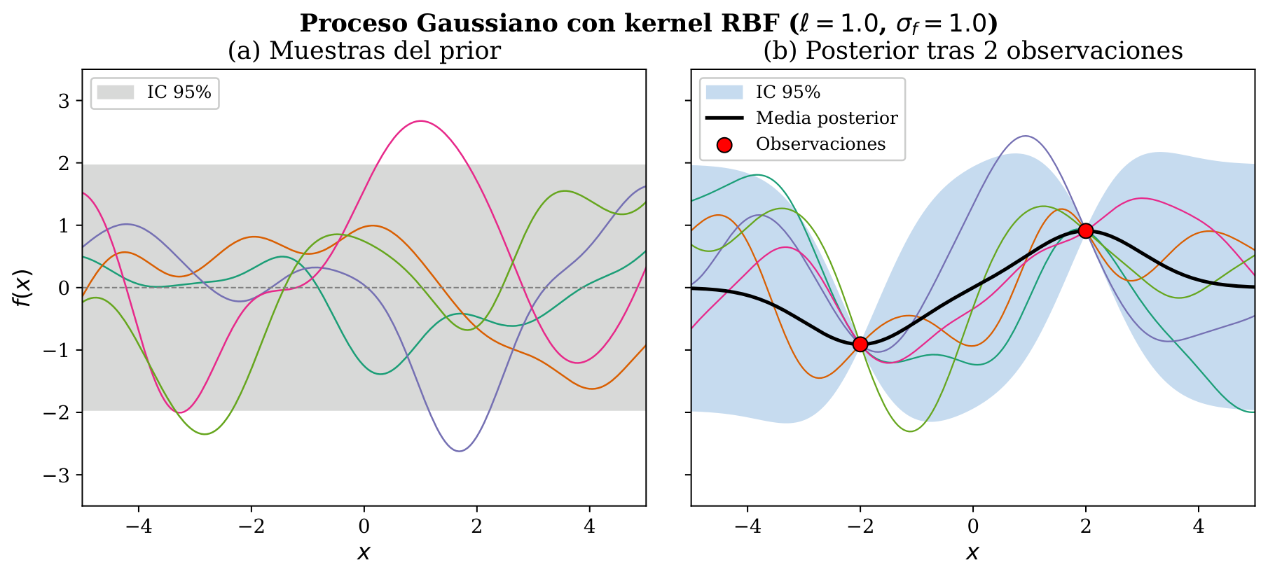
Following mainly Rasmussen and Williams (Rasmussen and Williams 2006), this subsection introduces the GP as a Bayesian non-parametric regression model. Its interest in the context of probabilistic surrogate models lies in the fact that, in addition to providing a mean prediction, it offers an analytical quantification of uncertainty, essential in Bayesian optimization (BO). To that end, the definition of the GP as a distribution over functions will be presented first, followed by its interpretation from Bayesian linear regression in feature space. Figure 2.1 illustrates this idea by showing the transition from a prior distribution over functions to a posterior distribution after observing data.

Definition and consistency

Formally, a GP is a stochastic process defined over the input space $\mathcal{X}$ such that, for any finite set of points $X=\{x_1,\dots,x_n\}\subset\mathcal{X}$, the vector of function values

$$\mathbf{f}_X = \bigl(f(x_1),\dots,f(x_n)\bigr)^\top$$

follows a multivariate normal distribution. Consequently, there exists a mean function $m:\mathcal{X}\to\mathbb{R}$ and a covariance function $k:\mathcal{X}\times\mathcal{X}\to\mathbb{R}$ such that

$$\mathbf{f}_X \sim \mathcal{N}\!\bigl(\mathbf{m}_X,\mathbf{K}_{XX}\bigr),$$

where

$$\mathbf{m}_X = \begin{bmatrix} m(x_1)\\ \vdots\\ m(x_n) \end{bmatrix}, \qquad (\mathbf{K}_{XX})_{ij}=k(x_i,x_j).$$

In shorthand, this is written as

$$f(x)\sim \mathcal{GP}\!\bigl(m(x),k(x,x')\bigr).$$

The above expression defines the GP prior over any finite set of points. Therefore, specifying a Gaussian process amounts to fixing two objects: a mean function $m(x)$, which captures the expected global trend of the function, and a covariance function $k(x,x')$, also called a kernel, which determines how the function values at different points of the domain relate to one another.

The choice of the mean function is part of the prior specification. In general, a GP does not require zero mean; however, a common choice is to take $m(x)=0.$ This assumption is reasonable when there is no clear prior information about a global deterministic trend, since it allows most of the model’s structure to be delegated to the covariance function. Moreover, it arises naturally if one starts from a centered Bayesian linear model,

$$f(x)=\phi(x)^\top w, \qquad w\sim\mathcal{N}(0,\Sigma_p),$$

then the induced mean over the function satisfies

$$\mathbb{E}[f(x)] = \phi(x)^\top\mathbb{E}[w] = 0.$$

If a known or relevant trend existed, it could be incorporated through a non-zero mean function or through explicit basis functions.

Once the mean is fixed, the second element needed to define the prior is the covariance function $k(x,x')$, which induces the covariance matrix $\mathbf{K}_{XX}$, defined in the previous equation, which must be symmetric and positive semi-definite in order to represent a valid covariance. Intuitively, the kernel encodes the prior assumptions about the regularity, smoothness, and scale of variation of the unknown function.

In addition to defining mean and covariance, the Gaussian distributions associated with different finite subsets of the domain must be coherent with one another. This coherence is obtained thanks to a fundamental property of the multivariate Gaussian distribution: consistency under marginalization.

Proposition: marginalization of a multivariate Gaussian.

Let

$$\begin{bmatrix} \mathbf{f}_A\\ \mathbf{f}_B \end{bmatrix} \sim \mathcal{N}\!\left( \begin{bmatrix} \boldsymbol{\mu}_A\\ \boldsymbol{\mu}_B \end{bmatrix}, \begin{bmatrix} \Sigma_{AA} & \Sigma_{AB}\\ \Sigma_{BA} & \Sigma_{BB} \end{bmatrix} \right),$$

where $\mathbf{f}_A$ and $\mathbf{f}_B$ are two subvectors of the joint Gaussian vector. Then, the marginal distribution of $\mathbf{f}_A$ is given by

$$\mathbf{f}_A \sim \mathcal{N}(\boldsymbol{\mu}_A,\Sigma_{AA}).$$

In this block partition, $\Sigma_{AA}$ is the covariance submatrix associated exclusively with the components of $\mathbf{f}_A$, while $\Sigma_{AB}$ and $\Sigma_{BA}$ capture the cross-covariances between $\mathbf{f}_A$ and $\mathbf{f}_B$.

This property guarantees that, although the GP is defined over a potentially infinite domain, inference can be performed exactly using only a finite number of points. In particular, it suffices to consider the joint distribution of the observed values and, where applicable, of the prediction points, since any subset of the process’s variables still follows a Gaussian distribution coherent with the overall specification.

The above definition introduces the GP directly in function space (function-space view): a prior is specified through its mean and covariance function, and consistency under marginalization guarantees the coherence of all the induced finite distributions. However, this formulation does not yet clearly show where the kernel comes from or how the model’s learning should be interpreted. For this, it is useful to return to a more familiar construction: Bayesian linear regression in a feature space, from which the GP appears when marginalizing the weights.

From weight space to function space

To understand more precisely the origin of the kernel and the meaning of learning in a GP, it is useful to start from classical Bayesian linear regression and observe how one transitions from a model defined by explicit parameters (weight-space view) to a formulation based solely on covariances between data (function-space view). Consider a latent function modeled as a linear combination of basis functions:

$$f(\bm{x}) = \bm{\phi}(\bm{x})^\top \bm{w},$$

where $\bm{\phi}(\bm{x})\in\mathbb{R}^N$ represents the feature vector associated with the input $\bm{x}$ and $\bm{w}\in\mathbb{R}^N$ is the weight vector. Instead of assuming there is a single, unknown true value of $\bm{w}$ (frequentist approach), the Bayesian approach introduces uncertainty over these parameters through a Gaussian prior: $\bm{w}\sim\mathcal{N}(\bm{0},\bm{\Sigma}_p).$ Observations are not considered equal to the latent function, but rather noisy realizations of it. For each observed data point it is assumed that

$$y_i = f(\bm{x}_i)+\varepsilon_i, \qquad \varepsilon_i\sim\mathcal{N}(0,\sigma_n^2),$$

with independent and identically distributed Gaussian noise. If we define $\bm{y}=[y_1,\dots,y_n]^\top$ and the design matrix in feature space as

$$\bm{\Phi}= \begin{bmatrix} \bm{\phi}(\bm{x}_1) & \cdots & \bm{\phi}(\bm{x}_n) \end{bmatrix} \in\mathbb{R}^{N\times n},$$

then the probabilistic model for the observations can be written as

$$\bm{y}\mid X,\bm{w}\sim\mathcal{N}(\bm{\Phi}^\top\bm{w},\sigma_n^2\bm{I}).$$

In the weight-space view, learning from the data amounts to a Bayesian update of the distribution over $\bm{w}$. Applying Bayes’ rule,

$$p(\bm{w}\mid X,\bm{y}) \propto p(\bm{y}\mid X,\bm{w})\,p(\bm{w}),$$

and given that both the likelihood and the prior are Gaussian, the posterior is Gaussian as well. Specifically,

$$p(\bm{w}\mid X,\bm{y})= \mathcal{N}(\bar{\bm{w}},\bm{A}^{-1}), \qquad \bm{A}=\sigma_n^{-2}\bm{\Phi}\bm{\Phi}^\top+\bm{\Sigma}_p^{-1}, \qquad \bar{\bm{w}}=\sigma_n^{-2}\bm{A}^{-1}\bm{\Phi}\bm{y}.$$

This expression summarizes what learning means in the weight-space view: the data do not fix a single weight vector, but rather update the probability distribution over them. The posterior mean $\bar{\bm{w}}$ represents the most plausible location of the weights after observing the data, while $\bm{A}^{-1}$ quantifies the residual uncertainty about those parameters.

From this posterior, a predictive distribution can already be obtained for a new point $\bm{x}_*$. Indeed, if $f_* = f(\bm{x}_*)=\bm{\phi}(\bm{x}_*)^\top \bm{w},$ then the predictive is obtained by marginalizing the uncertainty over $\bm{w}$:

$$p(f_*\mid \bm{x}_*,X,\bm{y}) = \int p(f_*\mid \bm{x}_*,\bm{w})\,p(\bm{w}\mid X,\bm{y})\,d\bm{w}.$$

Since $f_*$ is a linear transformation of a Gaussian variable, this distribution is also Gaussian:

$$p(f_*\mid \bm{x}_*,X,\bm{y}) = \mathcal{N}\!\Bigl( \bm{\phi}(\bm{x}_*)^\top \bar{\bm{w}}, \; \bm{\phi}(\bm{x}_*)^\top \bm{A}^{-1}\bm{\phi}(\bm{x}_*) \Bigr).$$

This formulation explicitly shows how the uncertainty over the weights propagates to the prediction. However, it also reveals a limitation: the inference depends on $\bm{A}^{-1}$, a matrix of size $N\times N$, where $N$ is the dimension of the feature space. If this space is very large or even infinite, this representation ceases to be operational. The decisive step then consists of rewriting the model solely in terms of inner products between features.

In fact, under the Gaussian prior over $\bm{w}$, the latent function evaluated at any point $\bm{x}$ is also a Gaussian random variable, since it is a linear combination of Gaussian variables. Therefore, for any finite set of inputs, the joint distribution of the function values is fully determined by its mean and covariance. In particular,

$$\mathbb{E}[f(\bm{x})] = \mathbb{E}[\bm{\phi}(\bm{x})^\top\bm{w}] = \bm{\phi}(\bm{x})^\top\mathbb{E}[\bm{w}] = 0,$$

and, for two arbitrary points $\bm{x}$ and $\bm{x}'$,

$$\operatorname{cov}\bigl(f(\bm{x}),f(\bm{x}')\bigr) = \mathbb{E}\!\left[ \bm{\phi}(\bm{x})^\top \bm{w}\bm{w}^\top \bm{\phi}(\bm{x}') \right] = \bm{\phi}(\bm{x})^\top \bm{\Sigma}_p \bm{\phi}(\bm{x}').$$

The dependence on the weights and their covariance can be grouped into a single function defined over pairs of inputs: $k(\bm{x},\bm{x}') = \bm{\phi}(\bm{x})^\top \bm{\Sigma}_p \bm{\phi}(\bm{x}').$ Thus, the uncertainty originally modeled over the parameters $\bm{w}$ is transferred to the covariance structure between function values.

From this perspective, for any finite set $X=\{\bm{x}_1,\dots,\bm{x}_n\}$, the vector of latent values $\bm{f}_X = \bigl(f(\bm{x}_1),\dots,f(\bm{x}_n)\bigr)^\top$ can be obtained by marginalizing the weights:

$$p(\bm{f}_X\mid X) = \int p(\bm{f}_X\mid X,\bm{w})\,p(\bm{w})\,d\bm{w}.$$

Since $\bm{f}_X=\bm{\Phi}^\top \bm{w}$ is a linear transformation of a Gaussian variable, its marginal distribution is also Gaussian, with

$$\mathbb{E}[\bm{f}_X]=\bm{0}, \qquad \operatorname{cov}(\bm{f}_X)=\bm{\Phi}^\top \bm{\Sigma}_p \bm{\Phi}=\bm{K}, \quad \text{with } K_{ij}=k(\bm{x}_i,\bm{x}_j).$$

Therefore,

$$\bm{f}_X \sim \mathcal{N}(\bm{0}_X,\bm{K}_X).$$

That is, marginalizing the weights directly yields a Gaussian distribution over the function values at any finite set of inputs. This is precisely the formulation of the GP in function space: the model ceases to be expressed in explicit terms of $\bm{w}$ and comes to be determined solely by its mean function and its covariance function.

The kernel trick

To connect the kernel trick with its functional interpretation, it is useful to draw on the theory of reproducing kernel Hilbert spaces. This part follows the presentation of kernel methods by Bishop (Bishop 2006) and the interpretation of RKHS and regularization by Hastie, Tibshirani and Friedman (Hastie et al. 2009).

The previous expression $k(\bm{x},\bm{x}') = \bm{\phi}(\bm{x})^\top \bm{\Sigma}_p \bm{\phi}(\bm{x}')$ shows that the covariance between two function evaluations does not depend explicitly on the weights $\bm{w}$, but only on how the inputs $\bm{x}$ and $\bm{x}'$ relate to each other in the feature space induced by $\bm{\phi}$ and weighted by $\bm{\Sigma}_p$. This is the point where the kernel trick comes in.

Since $\bm{\Sigma}_p$ is positive semidefinite, it can be written in terms of a matrix square root $\bm{\Sigma}_p^{1/2}$. Defining then a new feature map $\bm{\psi}(\bm{x})=\bm{\Sigma}_p^{1/2}\bm{\phi}(\bm{x}),$ the above covariance can be rewritten as

$$k(\bm{x},\bm{x}') = \bm{\psi}(\bm{x})^\top \bm{\psi}(\bm{x}').$$

Therefore, the kernel can be interpreted as an inner product in a transformed feature space. This observation has a fundamental consequence: if the model’s expressions depend only on inner products between transformed inputs, then it is not necessary to explicitly construct or manipulate the feature vector $\bm{\phi}(\bm{x})$. It suffices to have a function $k(\bm{x},\bm{x}')$ that directly returns that inner product.

Consequently, the model can operate implicitly in feature spaces of very high, or even infinite, dimension without abandoning a computable formulation. In the case of Gaussian processes, this means that inference and prediction can be expressed solely in terms of the kernel matrix $\bm{K}$, whose elements are $K_{ij}=k(\bm{x}_i,\bm{x}_j).$ The algebraic complexity thus ceases to depend on the explicit construction of the feature space and shifts instead to the handling of covariance matrices defined over the observed data.

From a conceptual standpoint, the kernel trick is not merely a computational simplification. It also makes it possible to separate two levels of modeling: on one hand, the choice of a kernel function $k$, which encodes prior hypotheses about smoothness, regularity, or structure of the unknown function; on the other, the concrete representation in terms of basis functions, which can remain implicit. This reformulation justifies that, once the GP has been introduced from Bayesian linear regression, the subsequent analysis can be developed entirely in terms of covariance functions.

RKHS and the representer theorem.

The above interpretation can be made precise through the concept of a reproducing kernel Hilbert space (RKHS). Given a symmetric, positive semidefinite kernel $k$, there exists a Hilbert space $\mathcal{H}_k$ formed by functions $f:\mathcal{X}\to\mathbb{R}$ in which each section $k(\cdot,\bm{x})$ belongs to the space and satisfies the reproducing property:

$$f(\bm{x})=\langle f,\;k(\cdot,\bm{x})\rangle_{\mathcal{H}_k}.$$

Moreover, the kernel itself satisfies

$$k(\bm{x},\bm{x}')= \langle k(\cdot,\bm{x}),\,k(\cdot,\bm{x}')\rangle_{\mathcal{H}_k}.$$

This property allows the kernel to be interpreted as an inner product in a feature space that may be of very high or infinite dimension. In the original space $\mathcal{X}$, the relationship between inputs and output may be nonlinear; however, through a suitable lift to a richer functional space, this relationship can be handled through linear operations in that new space. Within the RKHS framework, this lift is given canonically by $\Phi_k(\bm{x})=k(\cdot,\bm{x}),$ so that

$$k(\bm{x},\bm{x}')= \langle \Phi_k(\bm{x}),\Phi_k(\bm{x}')\rangle_{\mathcal{H}_k}.$$

Therefore, the kernel not only acts as a covariance function or as an implicit inner product, but also as the object that defines the geometry of the functional space in which the solution lives.

This interpretation reinforces the central idea of the kernel trick: it is not necessary to explicitly construct the lift $\Phi_k(\bm{x})$, which may be unknown or incomputable in practice, since the kernel allows one to work directly with the relevant inner products. Thus, the model can capture nonlinear relationships in the original space while implicitly working in a richer feature space.

The key structural result in this context is the representer theorem (Schölkopf et al. 2001). For a regularized learning problem of the form

$$J[f]=Q\bigl(y_1,\dots,y_n,f(\bm{x}_1),\dots,f(\bm{x}_n)\bigr) +\frac{\lambda}{2}\|f\|_{\mathcal{H}_k}^2,$$

where $Q$ measures the fit to the observed data, every minimizer $f\in \mathcal{H}_k$ can be written as a finite combination of kernels centered at the training points:

$$f(\bm{x})=\sum_{i=1}^n \alpha_i\,k(\bm{x},\bm{x}_i).$$

This result is especially important because it shows that, although $\mathcal{H}_k$ may be infinite-dimensional, the solution induced by a finite dataset lies within the subspace spanned by $\{k(\cdot,\bm{x}_1),\dots,k(\cdot,\bm{x}_n)\}.$

In the case of Gaussian processes, this same structure reappears in the predictive posterior mean, which can be written as a linear combination of kernel evaluations at the observed points. Thus, the probabilistic view of the GP and the functional view based on RKHS converge on the same idea: learning depends on the data only through the geometry induced by the kernel.

Covariance functions (Kernels)

The kernel encapsulates the prior assumptions about the smoothness, scale, and correlation structure of the latent function. For it to define a valid covariance matrix, it must be symmetric and positive semidefinite. In this work, the following kernels are considered:

• Linear (Dot Product). It is defined as

  $$k_{\mathrm{lin}}(\bm{x},\bm{x}') = \sigma_0^2 + \bm{x}^\top \bm{x}'.$$

  This kernel corresponds to a Bayesian linear regression in the original input space. The term $\bm{x}^\top\bm{x}'$ measures the linear similarity between two points, while $\sigma_0^2\geq 0$ acts as a bias or intercept term, allowing the function to be shifted relative to the origin. It is useful when the response is expected to show an approximately linear global trend.

• Squared Exponential (SE/RBF). It is expressed as

  $$k_{\mathrm{SE}}(\bm{x},\bm{x}') = \sigma_f^2 \exp\left( -\frac{1}{2}(\bm{x}-\bm{x}')^\top \bm{M} (\bm{x}-\bm{x}') \right).$$

  The parameter $\sigma_f^2>0$ is the signal variance and controls the vertical amplitude of the functions generated by the prior. The matrix $\bm{M}$ controls the scale of variation with respect to the input variables. In the isotropic case, $\bm{M}=\ell^{-2}\bm{I},$ where $\ell>0$ is the characteristic length-scale.

  In the ARD (Automatic Relevance Determination) case, it is common to use $\bm{M}=\mathrm{diag}(\ell_1^{-2},\dots,\ell_d^{-2}),$ allowing a different scale for each dimension. Small values of $\ell$ allow rapid variations of the function, while large values induce smoother functions with longer-range correlations.

  The SE/RBF kernel induces infinitely differentiable functions, which represents a very strong smoothness assumption. This property may be suitable for very regular responses, but it can also be excessive for physical phenomena with local changes, irregularities, or a lower degree of differentiability, where the model may oversmooth the real response.

• Matérn. The Matérn kernel generalizes the SE/RBF by introducing a smoothness parameter $\nu>0$, which controls the degree of differentiability of the generated functions. If $r=\|\bm{x}-\bm{x}'\|$ denotes the Euclidean distance between two inputs and $\ell>0$ the characteristic length-scale, the Matérn kernel is defined as

  $$k_{\text{Mat\'ern}}(r)= \sigma_f^2 \frac{2^{1-\nu}}{\Gamma(\nu)} \left(\frac{\sqrt{2\nu}\, r}{\ell}\right)^\nu K_\nu\left(\frac{\sqrt{2\nu}\, r}{\ell}\right).$$

  In this expression, $\Gamma(\nu)$ is the Gamma function, which generalizes the factorial to positive real values, and $K_\nu(\cdot)$ is the modified Bessel function of the second kind (NIST Digital Library of Mathematical Functions 2010). As with the SE kernel, $\sigma_f^2$ controls the amplitude of the function and $\ell$ determines the spatial scale of correlation. These parameters are not computed from a single closed-form formula, but are treated as kernel hyperparameters and fitted from the data, for example by maximizing the marginal log-likelihood (LML).

  The cases $\nu=3/2$ and $\nu=5/2$ are especially common because they yield simple closed-form expressions and allow the smoothness to be controlled more realistically than with the SE. In particular, $\nu=3/2$ induces less smooth functions, while $\nu=5/2$ allows for more regular functions, but without imposing the infinite smoothness of the SE/RBF kernel. For this reason, the Matérn kernel is usually appropriate when one wants to model a continuous function that is not necessarily infinitely differentiable.

• White Noise Kernel (White Kernel).

  $$k_{\mathrm{White}}(\bm{x},\bm{x}') = \sigma_n^2 \delta_{\bm{x},\bm{x}'}.$$

  In this expression, $\sigma_n^2>0$ represents the observation noise variance and $\delta_{\bm{x},\bm{x}'}$ is the Kronecker delta, which equals $1$ when the inputs coincide and $0$ otherwise. This kernel does not model a smooth structure of the latent function, but independent variability associated with the observations.

  If the observed model is written as

  $$y_i = f(\bm{x}_i)+\varepsilon_i, \qquad \varepsilon_i\sim\mathcal{N}(0,\sigma_n^2),$$

  then the covariance of the observations is not only the covariance of the latent function, but

  $$\operatorname{cov}(y_i,y_j) = k_f(\bm{x}_i,\bm{x}_j) + \sigma_n^2\delta_{ij}.$$

  Therefore, the white noise kernel is usually added to another kernel, such as RBF or Matérn, to represent that each observation may contain measurement error or independent numerical noise, without introducing spatial correlation between distinct points.

Isotropy and Automatic Relevance Determination (ARD). A kernel is said to be isotropic if the correlation depends only on the Euclidean distance $\|\bm{x}-\bm{x}'\|$, assuming that the function varies in the same way in all directions. However, in engineering problems it is common for some input variables to have a much greater influence on the response than others.

To capture this, we use ARD by defining the scale matrix $\bm{M} = \mathrm{diag}(\ell_1^{-2}, \dots, \ell_d^{-2})$. The parameters $\ell_d$ are the characteristic length-scales, which admit a direct physical interpretation:

• If $\ell_d$ is small, the function varies rapidly in that dimension (highly relevant variable).

• If $\ell_d$ is very large ($\ell_d \to \infty$), the function is nearly constant in that direction (irrelevant variable), effectively eliminating the dependence.

Prediction and uncertainty

Given a set of noisy observations $\mathcal{D}_n=\{(\bm{x}_i,y_i)\}_{i=1}^n,$ the observation model is assumed to be

$$y_i=f(\bm{x}_i)+\varepsilon_i, \qquad \varepsilon_i\sim\mathcal{N}(0,\sigma_n^2),$$

with independent Gaussian noise. In this subsection, we consider the prediction of the latent value of the function at a new test point $\bm{x}_*$, denoted by $f_* := f(\bm{x}_*).$

For simplicity, and in accordance with the zero-mean justification introduced in Section 2.2.1, we take $m(\bm{x})=0$. This assumption can be relaxed by incorporating a nonzero mean function when prior information about a global trend of the function is available. Under this convention, and using the consistency of finite Gaussian distributions described in the previous proposition, the joint distribution of the observations $\bm{y}$ and the latent value $f_*$ is given by

$$\begin{bmatrix} \bm{y} \\ f_* \end{bmatrix} \sim \mathcal{N}\left( \bm{0}, \begin{bmatrix} \bm{K}+\sigma_n^2\bm{I} & \bm{k}_* \\ \bm{k}_*^\top & k_{**} \end{bmatrix} \right).$$

In this expression, $\bm{K}=K(X,X)\in\mathbb{R}^{n\times n}$ is the kernel matrix between the training points, with entries $K_{ij}=k(\bm{x}_i,\bm{x}_j).$ The vector $\bm{k}_*=K(X,\bm{x}_*)\in\mathbb{R}^n$ collects the covariances between the observed points and the test point:

$$\bm{k}_* = \begin{bmatrix} k(\bm{x}_1,\bm{x}_*) \\ \vdots \\ k(\bm{x}_n,\bm{x}_*) \end{bmatrix},$$

while $k_{**}=k(\bm{x}_*,\bm{x}_*)$ is the prior variance of the latent function at $\bm{x}_*$. The term $\sigma_n^2\bm{I}$ appears only in the block corresponding to the observations $\bm{y}$, since these include measurement noise, while $f_*$ represents the noise-free latent value of the function.

Applying the conditioning rules of a multivariate Gaussian (Rasmussen and Williams 2006), we obtain the predictive posterior distribution

$$p(f_*\mid X,\bm{y},\bm{x}_*) = \mathcal{N}(\bar{f}_*,\mathbb{V}[f_*]),$$

where

$$\begin{aligned} \bar{f}_* &= \bm{k}_*^\top (\bm{K}+\sigma_n^2\bm{I})^{-1} \bm{y}, \\ \mathbb{V}[f_*] &= k_{**} - \bm{k}_*^\top (\bm{K}+\sigma_n^2\bm{I})^{-1} \bm{k}_*. \end{aligned}$$

The first equation provides the predictive posterior mean, that is, the average estimate of the latent value of the function at $\bm{x}_*$ under the model. The second quantifies the posterior uncertainty about that latent value. It is important to distinguish this posterior uncertainty about $f_*$ from the noise variance $\sigma_n^2$. The former reflects the model’s uncertainty about the latent function and can be reduced by incorporating informative observations. However, when the observations are very noisy, this uncertainty can remain high even in already evaluated regions, especially if there are not enough replicates or if the noise dominates the signal. If one wished to predict a new noisy observation $y_*$, rather than only the latent value $f_*$, the predictive variance should also include the noise term $\sigma_n^2$.

Training: parameter inference

In parametric point-estimation models, training usually consists of selecting a specific value of the model parameters, for example via maximum likelihood (MLE) or by minimizing a regularized loss function. From a Bayesian perspective, however, parameters can be treated as random variables: a prior is defined over them and, after observing the data, a posterior distribution is obtained. If one subsequently wishes to choose a single representative value for those parameters, one possible option is the MAP estimator. Nevertheless, in Gaussian process regression it is common to marginalize the weights or latent values and fit the parameters by maximizing the marginal likelihood.

In the case of Gaussian processes, training takes a different form than in classical parametric models. As seen in Section 2.2.2.0.1, the weights $\bm{w}$ of the feature-space representation are marginalized out, and their effect ends up encoded in the kernel. Therefore, training a GP does not consist of fixing a covariance family and estimating the hyperparameters that define it, together with the model’s noise level (Rasmussen and Williams 2006). In practice, a common strategy consists of maximizing the marginal likelihood of the data,

$$\hat{\bm{\theta}} = \arg\max_{\bm{\theta}} \log p(\bm{y}\mid X,\bm{\theta}).$$

This procedure is known as marginal likelihood maximization or type-II maximum likelihood. If, in addition, an explicit prior $p(\bm{\theta})$ over the parameters is introduced, then the corresponding criterion would be a MAP over $\bm{\theta}$:

$$\hat{\bm{\theta}}_{\mathrm{MAP}} = \arg\max_{\bm{\theta}} \left[ \log p(\bm{y}\mid X,\bm{\theta}) + \log p(\bm{\theta}) \right].$$

This work presents the standard formulation based on the LML, without including an additional prior on $\bm{\theta}$. The LML measures the probability of observing the training data under the model defined by the parameters $\bm{\theta}$. In GP regression with Gaussian noise, it is obtained by marginalizing the latent function values:

$$p(\bm{y}\mid X,\bm{\theta}) = \int p(\bm{y}\mid \bm{f},X,\bm{\theta})p(\bm{f}\mid X,\bm{\theta})\,d\bm{f}.$$

Since both the prior over $\bm{f}$ and the likelihood are Gaussian, this integral can be solved analytically and leads to:

$$\log p(\bm{y}\mid X,\bm{\theta}) = \underbrace{-\frac{1}{2}\bm{y}^\top \bm{K}_y^{-1}\bm{y}}_{\text{Data fit}} \quad \underbrace{-\frac{1}{2}\log|\bm{K}_y|}_{\text{Complexity penalty}} \quad \underbrace{-\frac{n}{2}\log 2\pi}_{\text{Constant}},$$

where $\bm{K}_y=\bm{K}_f+\sigma_n^2\bm{I}$ is the covariance matrix of the noisy observations.

The three terms in the expression above have complementary interpretations:

1. Data fit. The term $-\frac{1}{2}\bm{y}^\top \bm{K}_y^{-1}\bm{y}$ measures the compatibility between the observations and the covariance structure induced by the kernel. It can be interpreted as a Mahalanobis distance with respect to the model’s mean. It penalizes parameter configurations under which the observed data are unlikely.

2. Complexity penalty. The term $-\frac{1}{2}\log|\bm{K}_y|$ depends on the covariance matrix and, therefore, on the kernel and noise parameters. It acts as a complexity penalty: overly flexible models can assign probability to many possible patterns, diluting the probability assigned to the particular set of observed data. Conversely, excessively rigid models may fail to explain the data well.

3. Normalization constant. The term $-\frac{n}{2}\log 2\pi$ depends only on the number of observations and does not affect the optimization of $\bm{\theta}$, although it is part of the full Gaussian density.

This decomposition is related to the trade-off between model fit and complexity, though it should not be literally confused with the classic bias-variance-noise decomposition. In GPs, noise appears explicitly in $\bm{K}_y$ via $\sigma_n^2\bm{I}$, while the model’s flexibility is controlled by the kernel parameters.

Interpretation as Bayesian regularization Maximizing the LML naturally incorporates a form of Bayesian regularization. The fit term favors parameters that explain the observations well, while the term associated with the determinant penalizes models whose flexibility spreads probability mass across too many possible configurations. This effect is related to the so-called Bayesian Occam’s Razor: among models capable of explaining the data, the evidence tends to favor those that do so without introducing unnecessary complexity.

However, this regularization should not be interpreted as an absolute guarantee against overfitting, nor as a universal substitute for model validation. The LML evaluates the data under the assumptions of the GP and the chosen kernel. If the kernel family is misspecified, other criteria, such as cross-validation or comparison with alternative kernels, may be necessary to assess the model’s predictive capacity. Furthermore, the LML surface can present multiple local optima, so the result may depend on the optimizer’s initialization and on the kernel’s parametrization.

It is worth noting that regularization is not exclusive to a frequentist approach. For example, Ridge regression can be viewed both as the minimization of a penalized loss and as the MAP estimator of a Bayesian linear regression with a Gaussian prior over the weights. Indeed, if $p(\bm{w})=\mathcal{N}(\bm{0},\sigma_w^2\bm{I})$ and the observation noise has variance $\sigma_D^2$, the MAP leads to a penalty

$$\lambda\|\bm{w}\|^2, \qquad \lambda=\frac{\sigma_D^2}{\sigma_w^2}.$$

Therefore, the regularization term can be interpreted as a prior preference for models with small weights. The difference in the GP is not that all forms of regularization disappear, but rather that it becomes incorporated into the choice of functional prior, that is, into the kernel and its parameters.

Experimental design and initial sampling

The performance of SBO depends heavily on the quality of the initial set of observations $\mathcal{D}_n$. If the first points are concentrated in a small region of the domain $\mathcal{X}\subset\mathbb{R}^d$, the surrogate model has little information about the rest of the search space. In a GP, this directly affects the mean and the predictive variance, which can become heavily conditioned by poor initial coverage. For this reason, before starting the sequential optimization phase, it is common to employ DoE strategies aimed at covering the domain in a representative way.

Uniform random sampling is the simplest alternative, but it can generate local clusters and poorly explored regions, especially when the evaluation budget is limited. To reduce this problem, space-filling designs are used, whose goal is to distribute the initial points more uniformly within the domain (Forrester et al. 2008). Among the most common alternatives are Latin Hypercube Sampling (LHS) and Sobol sequences.

Latin Hypercube Sampling divides the range of each variable into $n$ intervals of equal probability and selects the points so that, in each dimension, there is exactly one sample per interval. This guarantees good marginal stratification, though not necessarily optimal geometric coverage in the multidimensional space.

In this work, Sobol sequences are used, a family of low-discrepancy quasi-Monte Carlo sequences (Sobol’ 1967). Unlike pseudorandom sampling, these sequences are deterministic and are designed to cover the unit hypercube more uniformly. Discrepancy intuitively measures the difference between the empirical distribution of the generated points and an ideal uniform distribution; therefore, a low-discrepancy sequence tends to leave fewer gaps and fewer clusters than pure random sampling.

This property is useful in the initial construction of the surrogate model, as it allows obtaining a stable initial coverage of the domain before applying adaptive criteria for selecting new evaluations. Moreover, being deterministic, Sobol sequences facilitate the reproducibility of the initial design.

Regarding the size of the initial design, a common rule of thumb in surrogate-based optimization is to take a number of points proportional to the problem’s dimension, for example $n=10d$, where $d$ is the dimension of the input vector (Jones et al. 1998). In problems with very costly evaluations, this number can be reduced to reserve more budget for the sequential optimization phase.

Selection of new evaluations

Once an initial surrogate model has been built from the DoE, the challenge arises of how to use it to find the global optimum of the original problem. In the literature there are three main approaches to address this task (Jiang et al. 2020):

1. Pure heuristics: Algorithms such as genetic or evolutionary ones that directly evaluate the black-box function. They require thousands of high-fidelity evaluations, which is infeasible under strict budgets.

2. Surrogate-assisted metaheuristics: Use the surrogate model to pre-evaluate and filter individuals within an evolutionary population before running the actual simulation. Although they reduce cost, their population-based nature still demands a considerable number of samples.

3. Surrogate-Based Optimization (SBO): This is the most efficient approach for costly problems. It relies on a probabilistic model to guide the search sequentially, evaluating a single point (or a small batch) at each iteration, maximizing the information gained.

Approach: sequential optimization with a limited budget

The SBO workflow, and particularly BO, is closely related to machine learning paradigms such as Active Learning, where the model actively selects which new observations would be most informative for improving its learning (Settles 2009). However, in the context of surrogate-based optimization it is more specifically referred to as the infill process, since the goal is not only to improve the model’s global accuracy, but to guide the search for the optimum under a limited evaluation budget $B$ by optimizing an acquisition function.

This function, which is much cheaper to evaluate, intelligently decides which is the optimal candidate $x^*$ for the next iteration. Once determined, it is evaluated on the (costly) real system, added to $\mathcal{D}_n$, and the surrogate model is retrained (updating its parameters). This cycle is repeated until the evaluation budget $B$ is exhausted or until a convergence criterion is satisfied.

Exploration vs exploitation

The design of the acquisition function defines the algorithm’s behavior, and it must balance two opposing forces (Jiang et al. 2020):

• Exploitation (Local search): Prioritize the regions of the search space where the surrogate model predicts that the objective function value is very good (minimum, in the case of minimization). A purely exploitative strategy converges quickly, but is highly susceptible to getting trapped in local minima.

• Exploration (Global search): Prioritize regions with high uncertainty, that is, where the model has little data and the predictive variance is high. A purely exploratory strategy behaves like pseudorandom sampling, wasting evaluations in unpromising areas.

Bayesian Optimization and acquisition functions

In BO, the selection of new evaluations is performed via acquisition functions, which use the surrogate model’s predictive distribution to decide which point should be evaluated next (Jones et al. 1998). Although various criteria exist, such as Probability of Improvement (PI), EI, or Lower Confidence Bound (LCB), in this work we will focus on EI, one of the most widely used criteria in BO for its ability to explicitly combine exploitation and uncertainty.

Probability of Improvement (PI) The PI criterion was one of the first developed. Its goal is to maximize the probability that a new point $\bm{x}$ improves upon the best solution observed so far, $f_{\min}$. If we assume that the prediction at $\bm{x}$ follows a normal distribution $\mathcal{N}(\mu(\bm{x}), \sigma^2(\bm{x}))$, the probability of improvement is:

$$PI(\bm{x}) = P(Y(\bm{x}) < f_{\min}) = \Phi\left( \frac{f_{\min}-\mu(\bm{x})}{\sigma(\bm{x})} \right),$$

where $\Phi$ is the cumulative distribution function of the standard normal.

The main limitation of PI is that it only accounts for the probability of improving the current value, but not the expected magnitude of that improvement. As a result, it can assign high value to points with a high probability of producing a very small improvement, biasing the search toward excessive local exploitation.

Expected Improvement (EI) Expected Improvement resolves this limitation by considering not only whether a point can improve upon the best observed value, but by how much it is expected to improve it (Jones et al. 1998). For a minimization problem, we define the improvement function relative to the current best observation $f_{\min}$ as:

$$I(\bm{x}) = \max(0, f_{\min}-Y(\bm{x})).$$

Equivalently, the function can be written piecewise:

$$I(\bm{x}) = \begin{cases} f_{\min}-Y(\bm{x}), & \text{if } Y(\bm{x})<f_{\min},\\ 0, & \text{if } Y(\bm{x})\geq f_{\min}. \end{cases}$$

Since $Y(\bm{x})$ is a random variable modeled by the GP, the expected improvement is obtained by integrating the improvement over the predictive density:

$$\mathbb{E}[I(\bm{x})] = \int_{-\infty}^{f_{\min}} (f_{\min}-y) \frac{1}{\sigma(\bm{x})} \phi\left( \frac{y-\mu(\bm{x})}{\sigma(\bm{x})} \right) \,dy,$$

where $\phi(\cdot)$ is the density function of the standard normal. Making the change of variable

$$z=\frac{y-\mu(\bm{x})}{\sigma(\bm{x})}, \qquad dy=\sigma(\bm{x})\,dz,$$

the upper limit becomes $Z=\frac{f_{\min}-\mu(\bm{x})}{\sigma(\bm{x})}.$ Therefore,

$$\mathbb{E}[I(\bm{x})] = \int_{-\infty}^{Z} \left(f_{\min}-\mu(\bm{x})-\sigma(\bm{x})z\right)\phi(z)\,dz.$$

Separating the terms:

$$\mathbb{E}[I(\bm{x})] = (f_{\min}-\mu(\bm{x}))\int_{-\infty}^{Z}\phi(z)\,dz - \sigma(\bm{x})\int_{-\infty}^{Z}z\phi(z)\,dz.$$

Since

$$\int_{-\infty}^{Z}\phi(z)\,dz=\Phi(Z), \qquad \int_{-\infty}^{Z}z\phi(z)\,dz=-\phi(Z),$$

we obtain the closed-form expression:

$$\mathbb{E}[I(\bm{x})] = \begin{cases} (f_{\min} - \mu(\bm{x})) \Phi(Z) + \sigma(\bm{x}) \phi(Z), & \text{if } \sigma(\bm{x}) > 0, \\[0.2em] 0, & \text{if } \sigma(\bm{x}) = 0, \end{cases} \qquad Z = \frac{f_{\min} - \mu(\bm{x})}{\sigma(\bm{x})}.$$

The closed-form expression of EI explicitly combines the two search strategies:

• The first term, $(f_{\min} - \mu(\bm{x})) \Phi(Z)$, dominates when the model predicts a low value of $\mu(\bm{x})$, that is, a better expected outcome in a minimization problem. This term drives exploitation of promising areas.

• The second term, $\sigma(\bm{x}) \phi(Z)$, dominates when the uncertainty $\sigma(\bm{x})$ is large, favoring exploration of regions where the model still has little information.

Mathematically, this synthesis of strategies can be demonstrated analytically by computing the partial derivatives of the EI function with respect to the model’s predictive moments. On the one hand, the derivative with respect to the predictive mean is:

$$\frac{\partial E[I(\bm{x})]}{\partial \mu(\bm{x})} = -\Phi(Z)$$

Since the cumulative distribution function $\Phi(Z)$ takes strictly positive values, this derivative is always negative. This shows that the EI function is monotonically decreasing with respect to $\mu(\bm{x})$. In practice, this means that the lower the value predicted by the model for a region—and therefore the better in a minimization problem—the greater its expected improvement, which pushes the algorithm to exploit promising areas.

On the other hand, the derivative with respect to the predictive uncertainty results in:

$$\frac{\partial E[I(\bm{x})]}{\partial \sigma(\bm{x})} = \phi(Z).$$

Since the standard normal density function $\phi(Z)$ is always greater than zero, this derivative is strictly positive. Consequently, EI is monotonically increasing with respect to $\sigma(\bm{x})$. Its practical meaning is that, given two locations with the same mean prediction, the algorithm will always assign a higher acquisition value to the one with greater uncertainty, thereby formalizing exploration. Greater uncertainty widens the variance of the predictive Gaussian bell, increasing the probability area that falls below the threshold $f_{\min}$.

At the design points already observed in the dataset (assuming noise-free observations), the GP’s certainty is absolute, i.e., $\sigma(\bm{x}) = 0$. Evaluating this limit, the expected improvement vanishes ($E[I(\bm{x})] = 0$). This property is critical, as it inherently prevents the algorithm from stagnating, ensuring that valuable computational budget is not wasted evaluating exactly the same point twice.

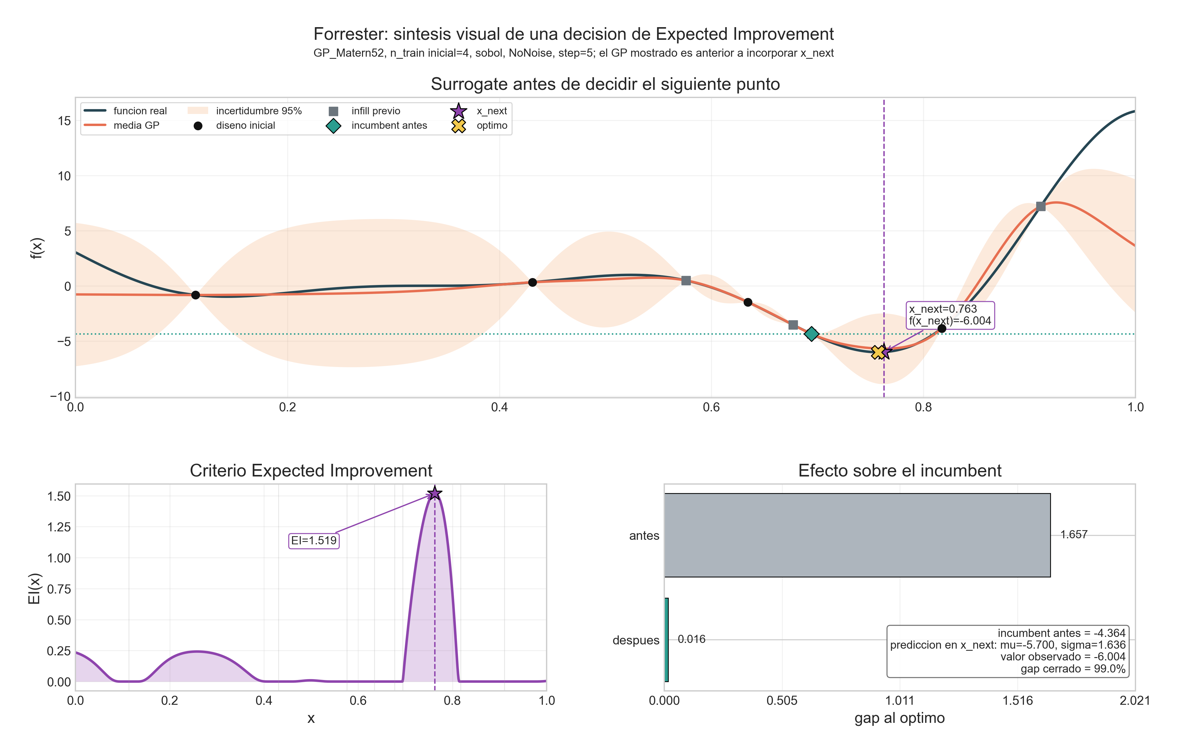
Taken together, these properties make EI suitable as a selection criterion within the infill process: it allows proposing new evaluations by combining the search in promising regions with the exploration of areas where the model still has uncertainty. This sequential mechanism will be used in the experimental part of the work and is summarized schematically in Figure 2.2.

Once the maximum evaluation budget (B) is exhausted, or a predefined convergence criterion is reached, the enrichment process is deemed complete.

Evaluation metrics

To validate the performance of surrogate models, it is not enough to evaluate the accuracy of their point predictions. In the case of probabilistic models such as Gaussian Processes, it is essential to quantify the quality of their predictive uncertainty. For this reason, the evaluation metrics are divided into two categories: classic predictive metrics and probabilistic metrics.

Predictive metrics (MAE, RMSE, R$^2$)

These metrics evaluate the divergence between the actual observation $y_i$ and the model’s predictive mean $\mu_i$ (or $\hat{y}_i$) over a set of size $N$.

• MAE (Mean Absolute Error): Given by $\text{MAE} = \frac{1}{N} \sum_{i=1}^{N} |y_i - \mu_i|$. It represents the average magnitude of prediction errors, without considering their direction. It grows linearly, which makes it more robust to outliers than RMSE.

• RMSE (Root Mean Squared Error): Defined as $\text{RMSE} = \sqrt{\frac{1}{N} \sum_{i=1}^{N} (y_i - \mu_i)^2}$. By squaring the differences, it severely penalizes large errors (outliers or disastrous predictions) compared to small errors.

• Coefficient of determination ($R^2$): Expressed as $R^2 = 1 - \frac{\sum_{i=1}^{N} (y_i - \mu_i)^2}{\sum_{i=1}^{N} (y_i - \bar{y})^2}$. It measures the proportion of the total variance of the dependent variable that is explained by the model.

Probabilistic metrics (NLL, NLPD)

While metrics such as RMSE, MAE, or $R^2$ evaluate only the quality of the point prediction, probabilistic metrics take into account the model’s full predictive distribution. In the case of a GP, this means evaluating not only whether the predictive mean $\mu_i$ approximates the observed value $y_i$, but also whether the uncertainty assigned by the model is consistent with the errors it makes.

This distinction is important in probabilistic surrogate models, since a good predictive mean does not guarantee good uncertainty quantification. A model can be accurate on average but overconfident; or it may cover almost all actual points through excessively wide, and therefore uninformative, intervals. For this reason, in addition to the classic predictive metrics, metrics based on predictive density and interval coverage are considered (Rasmussen and Williams 2006; Gneiting and Raftery 2007; Kuleshov et al. 2018).

Negative Log-Likelihood and Negative Log Predictive Density.

It is worth distinguishing between two related quantities that are used in different contexts. During GP training, it is common to minimize the negative of the LML, also called the negative log marginal likelihood: $-\log p(\bm{y}\mid X,\bm{\theta}),$ which corresponds to the opposite sign of the LML expression defined earlier. This quantity is used to fit the kernel and noise parameters $\bm{\theta}$.

By contrast, to evaluate probabilistic performance on a test set, it is more appropriate to use the Negative Log Predictive Density (NLPD). This metric evaluates, point by point, the probability that the trained model assigns to the actually observed value. If, for each test point $\bm{x}_i$, the predictive distribution is $p(y_i\mid \bm{x}_i,\mathcal{D}_n)=\mathcal{N}(\mu_i,s_i^2),$ then the average NLPD over a test set of $N$ samples is defined as

$$\mathrm{NLPD} = \frac{1}{N} \sum_{i=1}^{N} \left[ \frac{1}{2}\log(2\pi s_i^2) + \frac{(y_i-\mu_i)^2}{2s_i^2} \right].$$

Here $s_i^2$ represents the variance of the predictive distribution used to evaluate $y_i$. If noisy observations are evaluated, this variance must include both the uncertainty over the latent function and the observation noise variance. If, on the other hand, a noise-free latent function is evaluated directly, only the posterior variance over $f(\bm{x}_i)$ would be used. Lower NLPD values indicate a better predictive distribution. The above expression notably penalizes two undesirable situations:

1. Overconfidence. If the model assigns a very small variance $s_i^2$ but the mean $\mu_i$ is far from the actual value $y_i$, the quadratic term $\frac{(y_i-\mu_i)^2}{2s_i^2}$ grows rapidly. This penalizes models that produce narrow intervals but fail with large errors.

2. Underconfidence. If the model systematically assigns very large variances, it may cover many actual values, but the term $\frac{1}{2}\log(2\pi s_i^2)$ increases. This penalizes predictive distributions that are excessively wide and uninformative.

Therefore, NLPD does not measure only the error of the mean, but the balance between accuracy and uncertainty calibration.

Experimentation and results

This chapter carries the previous theoretical framework over to the experimental design of the work. The goal is to evaluate the use of GPs as probabilistic surrogate models to approximate a relationship between input configurations and a response of interest, especially in scenarios where evaluations are limited or costly.

The experimentation is organized into two scenarios. First, synthetic benchmark functions are used, where the objective function is known and can be evaluated at new points. This scenario allows the full surrogate-based optimization cycle to be studied: initial design, GP fitting, sequential point selection via an infill criterion, and updating of the observed set. Second, a real case is presented based on experimental data on insect diets. In this case, the observations come from trials already conducted and are grouped by diet, so the main goal is not to run new physical evaluations, but to validate whether the model generalizes to unseen diets.

Therefore, both scenarios share the same general surrogate modeling framework, but not the same experimental protocol: the benchmarks allow the sequential search process to be analyzed in a controlled setting, while the real case evaluates the feasibility of the approach before proposing a prospective phase of recommending new configurations.

Common surrogate modeling framework

In both scenarios, we start from a finite set of observations

$$\mathcal{D}_n = \{(\bm{x}_i, y_i)\}_{i=1}^{n},$$

where $\bm{x}_i \in \mathcal{X}$ represents a set of input data and $y_i$ the observed response. From this data, a surrogate model is trained whose goal is to approximate the relationship between inputs and outputs, providing predictions for inputs not included in the observation set and, in the case of Gaussian processes, an uncertainty estimate.

Data, models, and preprocessing

The inputs are organized into a design matrix $X \in \mathbb{R}^{n \times d}$, where $n$ is the number of observations and $d$ the dimension of the input space. The responses are collected in a vector $\bm{y} \in \mathbb{R}^{n}$. In the benchmarks, each observation corresponds to a controlled evaluation of a synthetic function. In the real case, each observation corresponds to an experimental measurement associated with a diet, so the training and evaluation partitions must respect that grouping to avoid information leakage between replicates of the same diet.

The experimental design compares a constant baseline and several GP configurations. Before fitting, the input variables are standardized using a z-score: each column is centered using the training set mean and divided by its standard deviation. This transformation is re-estimated within each partition or experimental iteration and then applied to the corresponding evaluation set, thereby avoiding the use of test information during fitting. In the real case, the additional transformations needed to represent the diets are described in Section 3.3.

The design compares a constant baseline and several GP families. Table 3.1 summarizes which models are used in each experiment and what role they play in the analysis. The baseline is interpreted as a minimum reference; the GPs are the probabilistic surrogate models analyzed. This description defines the experimental protocol; the specific classes and packages used to run it are described separately.

Family	Use	Role in the analysis
Dummy	Benchmarks and real case	Constant prediction computed from the training set responses. Serves as a minimum reference against models that do use the input variables.
Linear GP	Benchmarks and real case	GP with linear kernel and white noise term. Represents a hypothesis of an approximately linear relationship between inputs and response.
RBF GP	Benchmarks and real case	GP with RBF kernel and white noise term. Introduces a smooth, nonlinear hypothesis with a common length scale.
Matérn $3/2$ GP	Benchmarks and real case	GP with Matérn $3/2$ kernel and white noise term. Allows less smooth functions than RBF.
Matérn $5/2$ GP	Benchmarks and real case	GP with Matérn $5/2$ kernel and white noise term. Assumes a smoother response than Matérn $3/2$, but less restrictive than RBF.
Composite GP	Real case	GP with additive kernel linear + Matérn $5/2$ + white noise. Used to combine a global trend with a smooth nonlinear component in the experimental diet dataset.
ARD variant	Depends on protocol	Variant with a separate length scale per variable. In the benchmarks it is applied to RBF and Matérn $5/2$ when the dimension allows it; in the real case it is tested only on the best previous kernel for each combination of target and input representation.

Model families considered per experiment.

Probabilistic prediction and uncertainty

For a new configuration $\bm{x}$, the GP returns a predictive mean $\mu(\bm{x})$ and a standard deviation $\sigma(\bm{x})$. The mean is used as the point prediction and the standard deviation as a measure of uncertainty. In the benchmarks, this uncertainty is used actively within EI to select new evaluations. In the real case, it is used as an indicator of prediction reliability, without yet running a physical infill phase.

Implementation environment

The experiments were implemented in Python, using pandas and numpy for data manipulation, scikit-learn for model fitting and validation, scipy and scikit-optimize for numerical utilities and optimization, and matplotlib, seaborn, and plotly for generating figures.

In the implementation, the models were encapsulated in the DummySurrogateRegressor and GPSurrogateRegressor classes, the latter built on a Pipeline with StandardScaler and GaussianProcessRegressor.

The runs were performed on a machine with 64-bit Windows 10.0.26200, an Intel(R) Core(TM) Ultra 7 155H processor, 22 logical threads and 32 GB of RAM.

Experiment 1: synthetic benchmarks

As previously mentioned, the first experiment uses synthetic benchmark functions, in which the objective function can be evaluated at new points in the domain. This allows the full surrogate-based optimization cycle to be studied: initial design, GP fitting, selection of new evaluations via EI, and sequential updating of the observed set. The analysis focuses on the evolution of the best value found, predictive capability, and uncertainty as new observations are incorporated.

Selected benchmarks

Four benchmarks in global optimization and surrogate modeling are considered (Surjanovic and Bingham 2013; Forrester et al. 2008; Dixon and Szegö 1978; Morris et al. 1993), with a reasonable progression of difficulty, from low-dimensional problems with visual interpretation to higher-dimensional functions that must be analyzed mainly through metrics. The search domains are defined in the implementation and are used consistently for initial sampling, the test set, and acquisition criterion optimization. All this information is summarized in Table 3.2.

Benchmark	Dim.	Domain	Role in the experiment
Forrester	1	$x \in [0,1]$	One-dimensional case for visualizing GP fit, uncertainty, and EI behavior.
Branin	2	$x_1 \in [-5,10]$, $x_2 \in [0,15]$	Multimodal two-dimensional function, useful for analyzing point selection in a representable domain.
Hartmann6	6	$x_i \in [0,1]$, $i=1,\dots,6$	Higher-dimensional and multimodal benchmark, evaluated mainly through metrics.
Borehole	8	Heterogeneous eight-variable domain	Engineering-inspired problem for studying the method’s behavior in higher dimensions.

Benchmarks selected for the synthetic experiment.

Initial design, budget, and GP configurations

For each benchmark, an initial design is generated within the search domain, representing the information available before starting the sequential infill process. Two initial sampling strategies are compared, Sobol and uniform random sampling, along with three initial sizes:

$$n_{\text{train}} \in \{1,\; 1 \times d,\; 4 \times d\},$$

where $d$ is the benchmark’s dimension. The case $n_{\text{train}}=1$ allows observing the system’s behavior starting from an extreme situation with a single initial observation, while $1 \times d$ and $4 \times d$ represent designs scaled with the problem’s dimension.

Starting from the initial design, the infill process adds $5 \times d$ new points, subject to a maximum of 50 observations along the trajectory. Three noise conditions are also considered: noise-free evaluation and Gaussian noise with levels $0.5$ and $1.0$. The general configuration is summarized in Table 3.3, which fixes the common conditions later used to aggregate and compare results.

The detailed Borehole domain, the complete infill process flow, and the specific seed configuration are included as supplementary material in Appendix 5. Specifically, the Borehole domain is presented in Table 5.1, the sequential process diagram in Figure 5.1, and the seeds used in Table 5.2.

Element	Configuration
Benchmarks	Forrester, Branin, Hartmann6, and Borehole.
Initial sampling	Sobol and uniform random.
Initial size	$n_{\text{train}} = 1$, $1 \times d$, and $4 \times d$.
Infill budget	$5 \times d$ points added to the initial design, with a maximum of 50 observations during the process.
Noise	Noise-free and Gaussian noise with levels $0.5$ and $1.0$.
GP models	Linear, RBF, Matérn $3/2$, and Matérn $5/2$ families, described in Table 3.1; in dimensions greater than one, ARD variants for RBF and Matérn $5/2$ are also evaluated.
Test set	Independent set generated within each benchmark’s domain.
Seeds	Fixed seeds are used to ensure the experiment’s reproducibility. The detailed configuration is presented in Appendix 5.3.

General configuration of the benchmark experiment.

At each iteration, the GP is fitted with the available set of observations $\mathcal{D}_n$. Next, EI is computed over the search domain and the next point is selected as

$$\bm{x}_{\mathrm{next}} = \operatorname*{arg\,max}_{\bm{x}\in\mathcal{X}} (EI(\bm{x})).$$

Although the objective function is framed as a minimization problem, EI is maximized because it represents the expected improvement over the best value observed so far. In the implementation, EI maximization is approximated using Differential Evolution; details of the acquisition function optimization procedure are presented in Appendix 5.2.

The complete computational configuration for this experiment, including the test set size, the EI exploration parameter, the optimizer’s budget, and the seeds used, is documented in Appendix 8.1.

Benchmark experiment metrics

The predictive and probabilistic metrics used to evaluate the GP, such as MAE, RMSE, $R^2$, NLPD, and predictive interval coverage, follow the definitions introduced in Section 2.5. In this experiment they are used to analyze whether the infill process improves the model’s predictive capability, but the main focus is not purely predictive: it is also of interest to verify whether EI succeeds in finding lower values of the objective function.

From an optimization standpoint, the main quantity is the relative improvement of the minimum found during the infill process. The best value available up to an iteration $t$ is called the incumbent. When the global optimum $f^\star$ is known, this improvement is expressed as the relative reduction of the gap to the optimum. For this, we define $g_t = f_{\mathrm{best},t}^{\mathrm{clean}} - f^\star,$ where $f_{\mathrm{best},t}^{\mathrm{clean}}$ is the best clean value found up to iteration $t$. From this distance we compute

$$I_t = \frac{g_0 - g_t}{g_0},$$

where $g_0$ corresponds to the initial gap of the starting design. Values close to zero indicate little improvement over the initial design, while values close to one indicate an almost complete reduction of the initial distance to the optimum.

In Borehole, since no global optimum is defined in the implementation, no gap to the optimum is computed. In this case, the same reading is approximated through the relative reduction of the best clean value found compared to the initial design. Therefore, the text uses “relative improvement of the minimum found” as a general term, and “gap reduction” only when a reference optimum exists.

Besides the final improvement, the cumulative improvement during the trajectory is also considered. This quantity summarizes the evolution of the relative improvement throughout the infill process and allows distinguishing between configurations that find good solutions early and configurations that only improve toward the end of the available budget. Thus, the final improvement measures the outcome achieved at the end of the process, while the cumulative improvement provides a temporal reading of the search.

Predictive capability is analyzed through the relative MAE with respect to the initial state and through comparison against the Dummy model. Relative MAE allows checking whether the added observations reduce the GP’s error on an independent test set.

Probabilistic metrics, particularly NLPD and 95% coverage, are interpreted as a complementary diagnostic of uncertainty. Low NLPD values and coverages close to the nominal level indicate more coherent predictive distributions, although they do not by themselves guarantee a better search for the optimum.

Benchmark experiment results

The results are organized at three levels. First, whether the EI-based infill process improves the best value found of the objective function is analyzed. Then, whether the new observations also improve the GP’s predictive capability is studied. Finally, the experimental factors that most condition the observed performance are summarized, such as initial size, noise, dimensionality, kernel, and the use of ARD.

Evolution of the minimum found during the infill process

The main metric from an optimization standpoint is the relative improvement of the minimum found, defined in Section 3.2.3. In this analysis, step=0 represents the best point available in the initial design, before adding new evaluations. From there, each iteration incorporates the point selected by EI and updates the best value found.

Table 3.4 summarizes the best model for each benchmark according to the final improvement of the minimum found. The cumulative improvement is also included, allowing us to distinguish whether the improvement appears early during the trajectory or is concentrated at the end of the infill budget.

Cumulative improvement is computed from the area under the normalized relative improvement trajectory. Thus, it measures not only the final result but also how quickly the improvement appears. A ratio close to one indicates that most of the improvement is obtained early, while a lower ratio suggests a later improvement.

The results show that EI achieves positive improvements in all four benchmarks, though with varying intensity. Branin shows the clearest final improvement, with an average gap reduction close to $0.90$. Forrester also shows a substantial improvement, while in Borehole this reading corresponds to the relative reduction of the best clean value compared to the initial design, since no reference optimum is available. Hartmann6 is the most demanding scenario: improvement exists, but it is more moderate and requires a more informative initial design, consistent with its higher dimensionality.

Benchmark	Best model	Final improvement	Cum. improvement	Ratio	$n_{\text{train}}$	Reading
Borehole	$GP\_Linear$	$0.720$	$0.694$	$0.963$	$1$	Early and strong improvement.
Branin	$GP\_Matern52\_ARD$	$0.898$	$0.596$	$0.663$	$1$	Very high final improvement.
Forrester	$GP\_Matern52$	$0.737$	$0.390$	$0.530$	$4$	Strong improvement, but later.
Hartmann6	$GP\_RBF$	$0.434$	$0.304$	$0.701$	$24$	Moderate improvement in higher dimension.

Summary of the best optimization model per benchmark. The final improvement corresponds to the relative improvement of the minimum found at the end of the infill process; in benchmarks with a known optimum it equals the relative reduction of the gap to the optimum. The cumulative improvement summarizes the evolution over the trajectory.

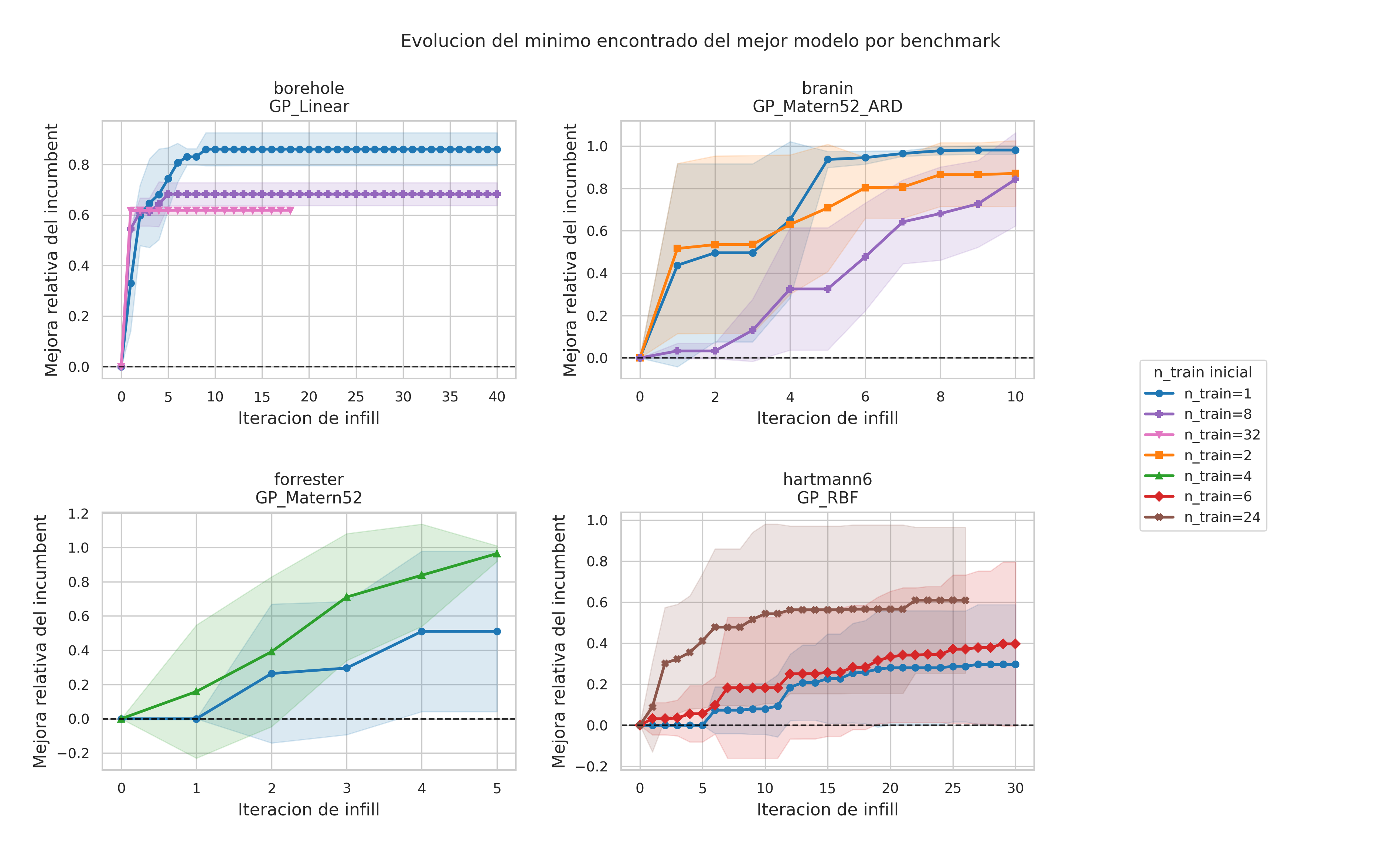
In Borehole, the final improvement and the cumulative improvement are very close, indicating that the process finds favorable regions from early stages. In Branin, the final improvement is very high, although part of the progress appears throughout the trajectory. Forrester shows a strong final improvement, but a less immediate one. In Hartmann6, progress is more gradual, confirming that the available budget is more restrictive in higher-dimensional problems.

Figure 3.1 confirms this temporal reading. In Borehole and Branin, much of the improvement appears during the early iterations and the curves then tend to stabilize. In Forrester, the trajectory depends more on the initial design and the improvement appears less immediately. In Hartmann6, progress is more gradual, reinforcing the importance of having more initial information in higher-dimensional problems. As supplementary material, Figure 5.2 shows the final relative improvement of the minimum found aggregated by benchmark.

Overall, the analysis of the relative improvement of the minimum found confirms that EI fulfills its main function within the optimization cycle: selecting new evaluations that improve the best value available compared to the initial design.

Evolution of the GP’s predictive capability

Besides success in optimization, we analyze whether the infill process improves the GP’s predictive capability. For this, the relative MAE with respect to the initial state is mainly used. This reading must be separated from the relative improvement of the minimum found: a configuration may predict better on average over the test set without necessarily being the most useful one for finding minima.

Table 3.5 summarizes the best predictive model for each benchmark and its comparison against Dummy. Dummy does not participate in the infill process, but serves as a reference to check whether the GP provides value compared to a trivial prediction.

Benchmark	Best MAE model	MAE improvement	Gain vs Dummy	% better than Dummy
Borehole	$GP\_RBF\_ARD$	$0.574$	$0.847$	$100.0\%$
Branin	$GP\_RBF$	$0.175$	$0.280$	$72.2\%$
Forrester	$GP\_RBF$	$0.281$	$0.291$	$66.7\%$
Hartmann6	$GP\_Linear$	$0.466$	$0.306$	$94.4\%$

Summary of the GP’s predictive improvement and comparison against Dummy.

The GP provides predictive value compared to Dummy across all benchmarks, though with varying intensity. The improvement is especially clear in Borehole and Hartmann6, while in Branin and Forrester it is more moderate and irregular. However, the best predictive models do not always coincide with the best optimization models. For example, in Hartmann6 the best model according to MAE is $GP\_Linear$, but the best model for improving the minimum found is $GP\_RBF$. Similarly, $GP\_RBF$ stands out in MAE for Branin and Forrester, while the best optimization models are $GP\_Matern52\_ARD$ and $GP\_Matern52$, respectively.

Las métricas probabilísticas se interpretan como diagnóstico complementario. En conjunto, el proceso de infill tiende a reducir simultáneamente el MAE y el NLPD respecto al estado inicial, aunque la calibración de la incertidumbre no es uniforme entre benchmarks. En Borehole y Branin se observa subcobertura en todos los modelos, lo que sugiere intervalos predictivos demasiado estrechos. En Forrester y Hartmann6 la cobertura se aproxima más al valor nominal en algunas configuraciones. Por tanto, la incertidumbre del GP resulta útil para guiar EI y diagnosticar la fiabilidad de las predicciones, pero no debe confundirse con una garantía directa de éxito en optimización.

Estos resultados confirman que la precisión global, la calibración probabilística y la utilidad para guiar la búsqueda del óptimo son aspectos relacionados, pero no equivalentes. Las figuras complementarias del Anexo 5 muestran con más detalle esta separación: RBF y Matérn concentran los comportamientos más estables en varios benchmarks, mientras que el kernel lineal resulta menos robusto y solo destaca en casos concretos; véanse las Figuras 5.3 y 5.4.

Influencia de las condiciones experimentales

Finalmente, se resume el efecto agregado de las condiciones experimentales evaluadas. Dado el elevado número de combinaciones, el objetivo no es describir cada configuración de forma aislada, sino identificar qué factores parecen condicionar más el rendimiento del proceso GP + EI.

Orden	Factor	Resultado observado	Conclusión
1	Benchmark y dimensionalidad	La mejor mejora final del incumbent cambia mucho entre funciones: Branin alcanza $0.898$, mientras que Hartmann6 queda en $0.434$.	La dificultad del paisaje objetivo domina el resultado. La dimensionalidad y la estructura de la función condicionan más que cualquier decisión aislada del pipeline.
2	$n_{\text{train}}$ inicial	El efecto del tamaño inicial es visible dentro de un mismo benchmark: el rango de mejora llega a $0.457$ en Forrester y $0.365$ en Branin.	La información inicial condiciona la trayectoria de EI. Con pocos puntos hay más margen de mejora relativa, pero también más inestabilidad; por eso debe leerse junto al valor final alcanzado.
3	Kernel	Las diferencias entre kernels no siempre son concluyentes. En Borehole varios modelos quedan prácticamente empatados, mientras que en Branin, Forrester y Hartmann6 destacan sobre todo variantes RBF y Matérn.	El kernel importa, pero no debe leerse como una competición con un único ganador. RBF y Matérn ofrecen el comportamiento más consistente, aunque la elección final depende de la geometría del benchmark y del criterio analizado.
4	ARD	En mejora del incumbent, ARD frente al kernel base da $\Delta=0.002$, con $46\%$ de pares favorables ($n=108$). En MAE el efecto es mayor: $\Delta=0.109$, $63\%$ favorable.	ARD no mejora de forma sistemática la optimización, aunque puede ayudar a la calidad predictiva. Su utilidad depende del benchmark y no debe presentarse como ventaja general.
5	Sampler	Sobol frente a random da $\Delta=0.035$ en incumbent, pero solo $38\%$ de pares favorables ($n=186$). En MAE, el delta es negativo.	El sampler tiene un efecto secundario e irregular. Puede cambiar trayectorias concretas, pero no aparece como factor dominante frente al benchmark, el tamaño inicial o el kernel.
6	Ruido	Comparando sin ruido frente a ruido gaussiano, el incumbent mejora en media: $\Delta=0.110$ para $\sigma=0.5$ y $\Delta=0.125$ para $\sigma=1.0$. Sin embargo, los porcentajes favorables son moderados.	El ruido reduce la estabilidad del proceso y puede degradar la búsqueda, pero su efecto no es uniforme. Depende del benchmark y de si se analiza optimización o calidad predictiva.

Lectura cualitativa de los factores que condicionan el rendimiento en benchmarks.

El Cuadro 3.6 no debe interpretarse como un ranking estadístico estricto, sino como una síntesis empírica de los patrones observados. La métrica principal para ordenar los factores es la mejora relativa final del mínimo observado, es decir, cuánto mejora el mejor valor encontrado tras el proceso de infill. Cuando se indican deltas, estos proceden de comparaciones emparejadas: por ejemplo, $\Delta>0$ en “Sobol — random” significa que Sobol obtiene mayor mejora media que random bajo las mismas condiciones restantes. La conclusión principal es que el rendimiento del ciclo GP + EI está condicionado ante todo por el propio benchmark. En una lectura práctica, el foco debe ponerse primero en la dificultad geométrica del problema, el tamaño del diseño inicial y la familia de kernel; ARD, el sampler y el ruido se interpretan como factores secundarios, capaces de modificar trayectorias concretas pero no de compensar por sí solos un problema mal condicionado o con poca información inicial. El análisis de los efectos de estas condiciones se recoge como material complementario en la Figura 5.5.

Experimento 2: caso real con dietas para insectos

El segundo experimento traslada el marco de modelos sustitutos a un caso real basado en datos experimentales de cría de insectos. En este contexto, el interés se centra en la fase larvaria, ya que es la fase utilizada posteriormente como fuente de alimentación. El problema experimental consiste en estudiar cómo distintas formulaciones de dieta afectan al crecimiento de las larvas y a su composición final.

El diseño experimental parte de una dieta control, compuesta únicamente por salvado de trigo. Esta dieta representa la referencia habitual de cría y permite comparar el efecto de introducir dietas no convencionales. Las dietas no convencionales mantienen el salvado de trigo como base, pero sustituyen una parte por un subproducto alimentario con valor nutricional. En el estudio principal se consideran tres subproductos: hoja de olivo, cascarilla de quinoa y orujo de oliva.

Desde el punto de vista del modelado, el objetivo no es únicamente ajustar un modelo a una tabla de datos, sino evaluar si un GP puede capturar relaciones útiles entre la composición de la dieta y la respuesta observada en las larvas. Estas relaciones son relevantes porque los ensayos físicos son limitados y cada nueva formulación requiere una validación experimental. Por tanto, el modelo sustituto se plantea como una herramienta previa para estimar respuestas y cuantificar incertidumbre antes de una posible fase prospectiva de selección de nuevas dietas.

Las respuestas de interés combinan parámetros productivos y variables de composición. En el plano productivo, una variable relevante es FCR, que mide la relación entre la cantidad de alimento consumido y la ganancia de peso obtenida. Valores menores de FCR indican una conversión más eficiente del alimento en biomasa. En el plano composicional, se consideran variables como PROTEINA (%) y QUITINA (%). En las primeras pruebas también se consideró TPC que recoge la concentración de compuestos fenólicos totales en las larvas tras la cría y se utiliza como indicador adicional asociado al efecto de la dieta pero no se analizarán sus resultados por escasez de muestras.

En consecuencia, el caso real persigue dos objetivos metodológicos. En primer lugar, comprobar si el GP es capaz de generalizar a dietas no vistas a partir de variables de composición, inclusión y tipo de subproducto. En segundo lugar, analizar si la incertidumbre predictiva puede servir como señal de fiabilidad del modelo. A diferencia del experimento con benchmarks sintéticos, aquí no se ejecuta un ciclo secuencial de infill, ya que las observaciones proceden de ensayos experimentales ya realizados.

Alcance del caso real y selección de Hermetia

El archivo experimental original contiene información para dos especies: Hermetia illucens y Tenebrio molitor. Además, recoge varios bloques de información: composición nutricional y TPC de las dietas, parámetros productivos de la cría, y composición nutricional y TPC de las larvas obtenidas. En este experimento se trabaja únicamente con el bloque experimental de Hermetia illucens.

Sin embargo, los datos de Tenebrio molitor no se han utilizado porque mezclan varios bloques experimentales, incorporan tipos adicionales de dieta y presentan diferencias de tratamiento, como el suministro de agua en algunos controles. Para mantener un caso cerrado y comparable, el análisis se limita a Hermetia illucens: 33 observaciones organizadas en 11 dietas con 3 réplicas por dieta. En este bloque, las variables de entrada están completas y los objetivos tienen disponibilidad suficiente: FCR cuenta con 31 valores válidos, mientras que quitina y proteína cuentan con 33.

Diseño experimental y dietas consideradas

El conjunto analizado contiene una dieta control, basada en salvado de trigo, y varias dietas no convencionales en las que parte de ese salvado se sustituye por hoja de olivo, orujo de oliva o cascarilla de quinoa. Para identificar las formulaciones se usan etiquetas breves que combinan el subproducto y el porcentaje de inclusión: por ejemplo, Hoja15 indica una dieta con un 15 % de hoja de olivo. La misma regla se aplica a las dietas con orujo y quinoa.

Cada formulación se ensayó en tres lotes independientes de larvas. Por ello, cada observación representa una réplica de una dieta, no una media por dieta. En la validación, las tres réplicas de una misma formulación se mantienen juntas: cuando una dieta se deja fuera, ninguna de sus réplicas participa en el entrenamiento. El Cuadro 3.7 resume el alcance del caso real.

Elemento	Descripción
Bloque analizado	Ensayos de Hermetia illucens
Observaciones	33 réplicas experimentales
Dietas evaluadas	11 formulaciones
Réplicas por dieta	3 lotes independientes
Dieta de referencia	Salvado de trigo sin inclusión de subproductos
Subproductos principales	Hoja de olivo, orujo de oliva y cascarilla de quinoa
Agrupación para validación	Réplicas de una misma dieta
Objetivos modelados	FCR, quitina y proteína larvaria
Nivel de trabajo	Réplica experimental

Resumen de los datos utilizados en el caso real.

La representación de entrada describe cada dieta mediante variables de formulación y composición. Se comparan dos conjuntos: uno reducido, con porcentaje de inclusión, proteína, fibra, grasa y TPC medios de la dieta; y otro completo, que añade cenizas, carbohidratos y ratios nutricionales derivados. En ambos casos se incluye el tipo de subproducto, de forma que el modelo distingue entre control, hoja de olivo, orujo de oliva y quinoa sin depender solo del nombre de la dieta.

De este modo, el modelo no utiliza únicamente el nombre de la dieta como identificador, sino una descripción estructurada de cada formulación. Esta representación permite estudiar si las variables disponibles contienen información suficiente para anticipar la respuesta de dietas completas no vistas durante el entrenamiento.

Limpieza y preprocesamiento

El dataset utilizado en el caso real se obtiene a partir del archivo experimental original mediante un proceso de limpieza, combinación y transformación de tablas. El objetivo de esta etapa es pasar de varias hojas de Excel, con información distribuida por tipo de análisis, a una tabla única a nivel de réplica experimental. En esa tabla, cada fila debe contener tanto la respuesta observada como las variables necesarias para describir la dieta evaluada.

El proceso seguido puede resumirse en los siguientes pasos.

Paso 1. Limpieza de las hojas originales.

En primer lugar, se normalizan las hojas correspondientes a composición de dieta, parámetros productivos, composición larvaria y TPC. Durante esta etapa se corrigen nombres de columnas duplicados, se homogeneizan tratamientos y se estructuran las columnas de medias y desviaciones. También se normalizan los nombres de las variables que se utilizarán posteriormente en el modelado.

Paso 2. Enumeración de réplicas.

Para poder unir correctamente las distintas fuentes de información, se asigna un identificador de réplica dentro de cada dieta. Este paso es necesario porque los parámetros productivos y la composición de larvas se registran a nivel de lote o réplica de cría. De este modo, cada observación final puede asociarse a una dieta concreta y a una réplica experimental concreta.

Paso 3. Construcción del dataset de productividad.

Una vez limpias las tablas originales, se construye el dataset de productividad de Hermetia. Para ello, se combinan los parámetros productivos con la composición larvaria usando como claves la dieta, el tratamiento, la réplica y la especie. Después, se añade la composición nutricional de la dieta y la información de TPC. El resultado es una tabla a nivel de réplica que integra información productiva, composición de larva y descripción de la dieta.

Paso 4. Extracción de metadatos de dieta.

A partir del nombre textual de cada dieta se generan variables estructuradas, como diet_name, byproduct_type e inclusion_pct. Esta transformación permite que el modelo no dependa únicamente del nombre de la dieta, sino de variables interpretables: tipo de subproducto, porcentaje de inclusión y composición nutricional. Además, se calculan ratios nutricionales derivados que se emplean en el modo completo de variables.

Paso 5. Selección del objetivo y filtrado de valores ausentes.

El modelado se realiza de forma independiente para cada variable objetivo. Para cada objetivo se eliminan únicamente las filas cuyo valor de respuesta está ausente. Esta decisión evita descartar observaciones válidas para el resto de objetivos. Así, FCR se evalúa con 31 observaciones válidas, mientras que QUITINA (%) y PROTEINA (%) se evalúan con las 33 observaciones disponibles.

Paso 6. Construcción de $X$, $\bm{y}$ y grupos.

Para cada objetivo se construye la matriz de entrada $X$, el vector de respuesta $\bm{y}$ y el vector de grupos. El vector $\bm{y}$ contiene los valores observados del objetivo seleccionado. El vector de grupos se construye a partir de diet_name, de forma que todas las réplicas de una misma dieta compartan el mismo identificador de grupo. Esta agrupación será la base del protocolo LODO descrito en la Sección 3.3.4.

Paso 7. Codificación de variables categóricas.

Las variables de entrada se forman combinando las variables numéricas seleccionadas con una codificación binaria del tipo de subproducto. En concreto, byproduct_type se transforma en variables indicadoras y se concatena con las variables numéricas del modo reducido o completo. Todas las columnas resultantes se convierten a formato numérico antes del ajuste del modelo.

Paso 8. Escalado dentro del Pipeline.

Variable scaling is performed within the Pipeline of each model. Therefore, the normalization parameters are estimated using only the training data of each partition and are then applied to the diet held out for testing.

In the final CSV used, the selected input variables do not present missing values. Overall, this preprocessing transforms the original experimental data into a supervised structure grouped by diet. This organization allows the model to be evaluated under a more demanding condition than a random row-wise partition: predicting the response of complete diets not observed during training.

Leave-One-Diet-Out Evaluation Protocol

The evaluation of the real case is carried out using a Leave-One-Diet-Out (LODO) protocol, motivated by the grouped structure of the dataset. The observations are not independent samples unrelated to one another, but rather experimental replicates associated with the same diet. Therefore, a random row-wise partition could place replicates of the same diet simultaneously in training and test, generating an overly optimistic estimate of the model’s predictive capacity.

Let $\mathcal{G}=\{g_1,\dots,g_K\}$ be the set of available diets. In the outer fold $k$, the test set is formed by all observations belonging to diet $g_k$:

$$\mathcal{D}_{\text{test}}^{(k)} = \{(\bm{x}_i,y_i): g_i = g_k\}.$$

The training set contains the remaining diets:

$$\mathcal{D}_{\text{train}}^{(k)} = \{(\bm{x}_i,y_i): g_i \in \mathcal{G}\setminus\{g_k\}\}.$$

In this way, all replicates of the held-out diet are excluded from fitting. In the Hermetia dataset, since there are 11 diets available, the protocol generates 11 outer folds.

Diagram of the LODO protocol: in each outer fold, a complete diet is reserved to measure final performance; hyperparameter selection is carried out through internal validation on the remaining diets.

Hyperparameter selection is performed in a nested manner. For each outer fold, the held-out diet is reserved exclusively for the final evaluation. On the remaining diets, an internal validation is run, also group-based, and the configuration with the lowest MAE is selected. The model is then retrained with all the observations from the outer training set and evaluated on the held-out diet.

This design evaluates a more demanding task than interpolating between replicates of already observed diets. The model must predict the response of a complete diet that has not participated in either the final fit or the hyperparameter selection. For this reason, the results obtained with LODO are interpreted as an estimate of the model’s ability to generalize to unseen diets within the available experimental space.

Models, fitting, and metrics

At this stage, the families from Table 3.1 corresponding to the real case are reused: Dummy, linear GP, RBF GP, Matérn $3/2$ GP, Matérn $5/2$ GP, and composite GP. All models are evaluated under the nested LODO protocol described in Section 3.3.4, independently for each target and for each input representation. To avoid excessive exploration of variants, ARD is not applied to all families from the start, but only to the best prior kernel for each combination of target and input representation; in the final protocol, this variant is limited to RBF or Matérn, not to the composite kernel.

The configuration necessary to reproduce both experiments is summarized jointly in Annex 8.

In the real case, the composite GP is specified as a sum of kernels:

$$k(\bm{x},\bm{x}') = C_1\,k_{\text{Lineal}}(\bm{x},\bm{x}') + C_2\,k_{\text{Matern }5/2}(\bm{x},\bm{x}') + k_{\text{White}}(\bm{x},\bm{x}'),$$

where $C_1$ and $C_2$ are positive scale constants. The linear component captures an overall trend of the response with respect to the input variables; the Matérn $5/2$ component allows smooth local deviations; and the white noise term represents experimental variability not explained by the available covariates.

The fitting process is organized into three levels:

Internal selection.

In each outer fold, the parameters are selected through an internal LODO applied only to the training diets. The selection metric is the MAE, so the configuration with the lowest MAE in internal validation is chosen.

External evaluation.

Once the parameters are selected, the model is retrained with all the diets from the outer training set and evaluated on the held-out diet. The final metrics come from this external evaluation, not from training. In the GP models, both the predictive mean and the standard deviation are obtained. This second quantity allows metrics associated with uncertainty to be computed.

The reading of the metrics relies on the predictive and probabilistic definitions introduced in Section 2.5, but in this case it is necessary to specify how they are aggregated under LODO validation. MAE is used as the main metric for selecting hyperparameters and comparing models, because it preserves the original units of each target and allows the mean error to be interpreted directly.

In LODO, each outer fold corresponds to a held-out diet. Therefore, the macro MAE is interpreted as the mean error per diet: it is calculated by averaging the MAE of the outer folds, so that each diet has the same weight. This is the main reading for the real case, since the goal is to evaluate generalization to complete unseen diets, not to favor diets with more valid replicates.

To compare models against the baseline, the relative MAE with respect to Dummy is used:

$$\rho_{\mathrm{Dummy}} = \frac{\mathrm{MAE}_{\mathrm{modelo}}}{\mathrm{MAE}_{\mathrm{Dummy}}}.$$

Values of $\rho_{\mathrm{Dummy}}<1$ indicate that the model reduces the error compared to the trivial prediction. In addition, when analyzing the difficulty of each held-out diet, the error is normalized by the range of the corresponding target. This normalization allows visual comparison of errors for variables with different scales, such as FCR, chitin, and protein.

In the GP models, predictive uncertainty is also evaluated. The coverage of the approximate 95% interval measures the proportion of observations falling within $\mu \pm 1.96\sigma$. In addition, the predictive standard deviation $\sigma(\bm{x})$ is compared with the observed absolute error $|y-\mu(\bm{x})|$, in order to check whether the model assigns greater uncertainty to the cases where it actually makes larger errors. These uncertainty metrics are not used to select parameters, but as a diagnostic of the GP’s reliability.

Finally, in the prospective part of the real case, EI is interpreted as an acquisition score rather than a validation metric. The observed incumbent represents the best diet already measured experimentally for each target, while the candidate with the highest EI is an untested formulation that the model considers informative due to its combination of predictive mean and uncertainty. This distinction avoids presenting a prospective recommendation as though it were a confirmed experimental result.

Real case results

The results of the real case are analyzed with a different reading than the benchmark experiment. In this scenario, only a limited set of already conducted experimental trials is available. Therefore, the main interest is not merely to measure the model’s mean error, but to check whether the GP learns relationships transferable to complete diets not observed during training.

Structural generalization versus memorization

The first question is whether the surrogate model extracts a general signal from the formulation and composition variables, or whether it only recognizes diets similar to those observed. For this, the LODO protocol described in Section 3.3.4 is used, which forces the model to predict a completely unseen formulation.

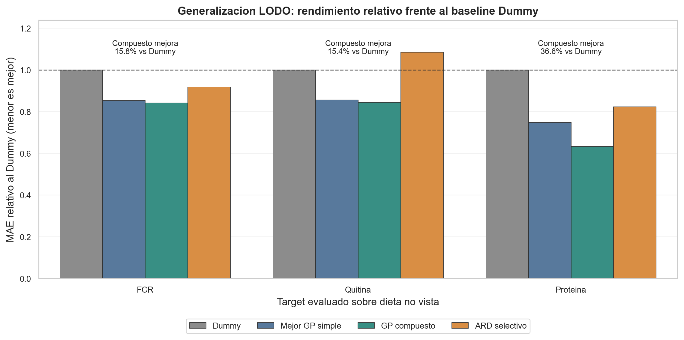
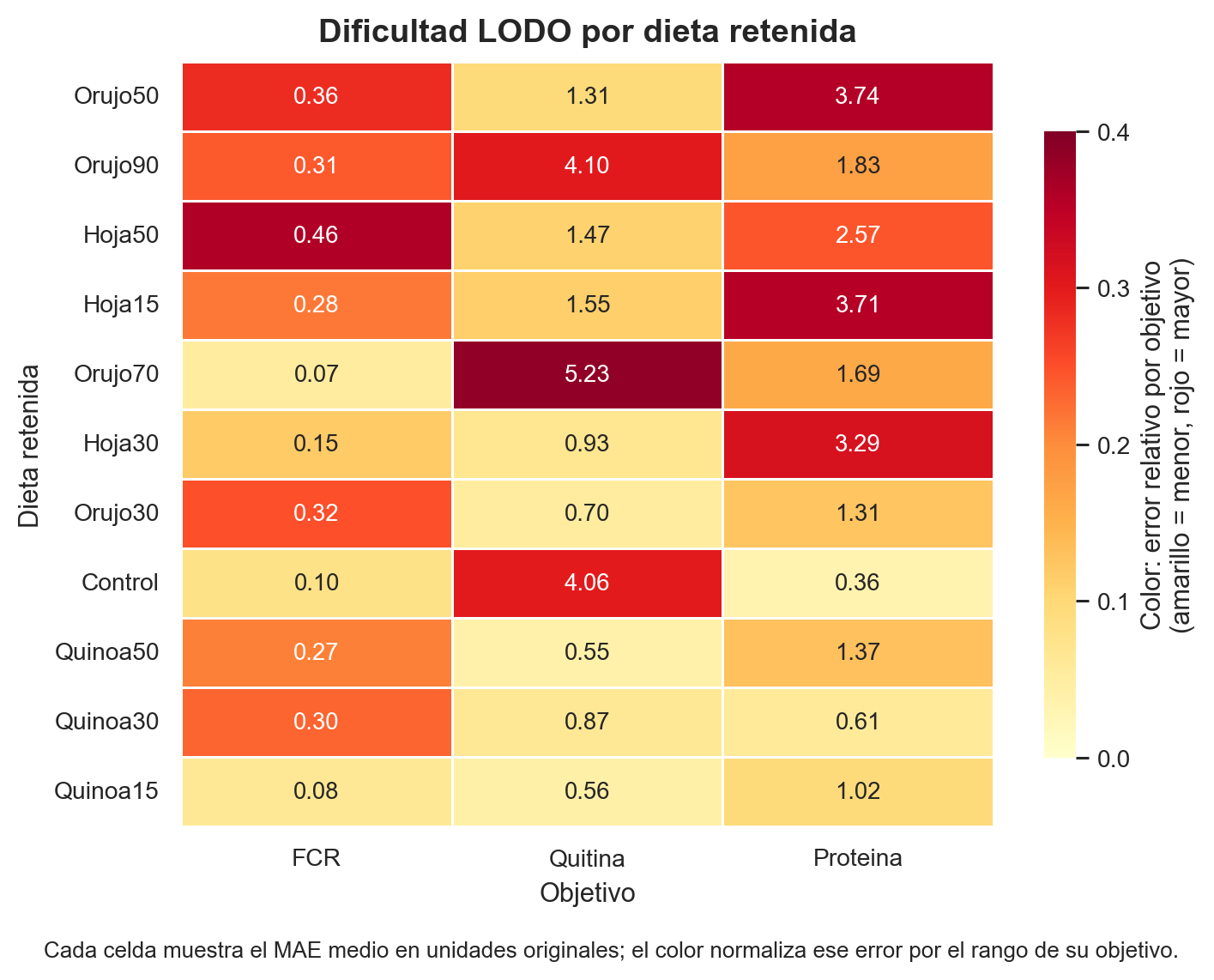
Figure 3.3 summarizes the relative performance against the Dummy model. The vertical axis represents the MAE normalized with respect to Dummy, so values below $1$ indicate improvement over the trivial prediction. Under this reading, the composite GP improves over Dummy on all three active targets: the relative error reduction is $15.8\%$ for FCR, $15.4\%$ for chitin, and $36.6\%$ for protein. This result indicates that the model is not limited to reproducing a global mean, but rather makes use of information contained in the input variables to anticipate, at least partially, the response of unseen diets.

However, this aggregate improvement should not be interpreted as uniform generalization. Figure 3.4 breaks down the error by held-out diet and shows that the difficulty of the problem depends on the formulation evaluated. In FCR, errors are relatively contained across several diets, although more difficult diets appear, such as Hoja50 and some formulations with pomace or quinoa. In chitin, difficulty is especially concentrated in diets such as Orujo70, Orujo90, and Control, while in protein, high errors stand out in diets such as Orujo50 and some leaf-based formulations.

The joint reading of both figures is important. The improvement over Dummy shows that there is a learnable signal in the nutritional and formulation variables, but the error map shows that this signal does not transfer equally to all diets. This is consistent with the nature of the real case: the larvae’s responses do not depend solely on an overall trend associated with the inclusion percentage or average composition, but also on effects specific to the byproduct, experimental variability, and possible interactions not fully represented in the available variables.

Consequently, the result does not allow us to claim that the GP fully solves the problem of predicting new diets. What it does allow is to argue that the composite model captures useful regularities beyond mere replicate memorization. LODO validation acts here as a test of structural generalization: if the model improves over Dummy when a complete diet is withheld, then part of the information learned comes from relationships shared between diets.

Geometric expressiveness of the composite GP

Once it has been verified that the GP provides predictive capacity relative to the baseline, the next question is what type of covariance structure is most appropriate for this real case. As explained in Section 2.2.3, the kernel is not merely a technical component of the GP, but the element that defines the prior hypotheses about the shape of the function to be approximated. In this case, the biological response of the larvae may contain an overall trend associated with the nutritional composition of the diet, but also local deviations due to the type of byproduct, the inclusion percentage, and experimental variability.

Figure 3.5 compares different kernel families using the mean MAE per diet, that is, the macro MAE of the LODO protocol. The comparison shows that the composite kernel is the most competitive model across the three targets considered. This difference is especially clear in protein, where the composite GP appreciably reduces the error compared to Dummy and to the simple kernels. In chitin, a consistent improvement is also observed relative to the individual alternatives, while in FCR the differences between several nonlinear kernels are smaller, although the composite kernel remains among the best options.

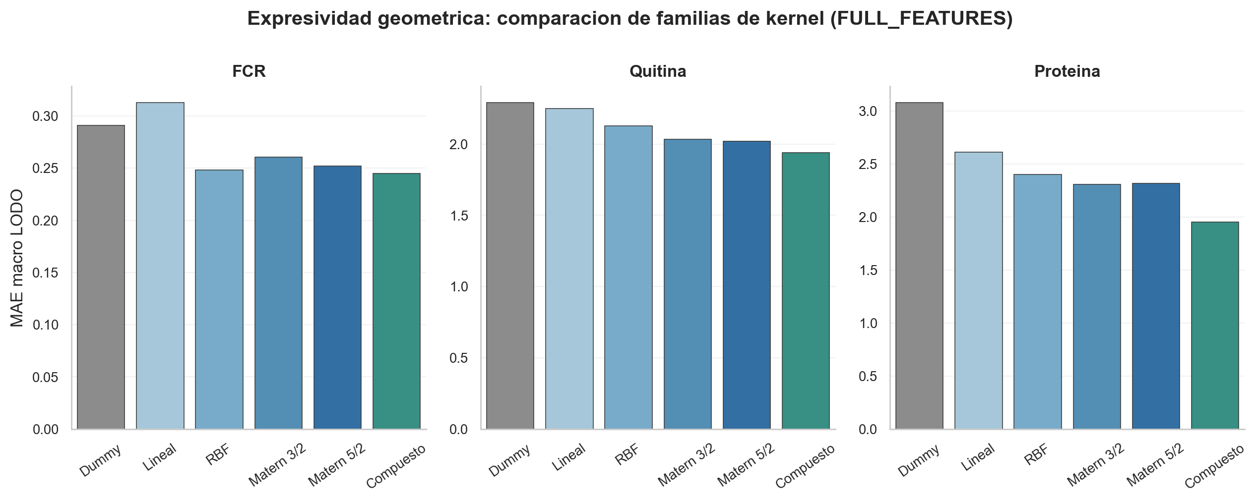
This reading is consistent with the previous definition of the composite GP: a covariance structure that combines an overall trend, local flexibility, and experimental noise. Therefore, the comparison in Figure 3.5 does not merely pit model names against each other, but rather different hypotheses about the shape of the relationship between diet and response.

Nevertheless, this result must be interpreted with caution. The superiority of the composite GP in Figure 3.5 does not mean that the model fully captures the biological dynamics of the system, nor that it can safely extrapolate beyond the observed experimental range. What it shows is that, within the space covered by the available diets and under LODO validation, a covariance structure combining overall trend, local variation, and experimental noise describes the data better than the simple families considered separately.

Therefore, the composite GP is adopted as the main model not because it eliminates the uncertainty of the real case, but because it offers the best observed combination of flexibility and robustness.

Practical calibration of uncertainty

In addition to evaluating the accuracy of the predictive mean, in this real case it is of interest to check whether the GP’s uncertainty provides useful information about the reliability of its predictions. This question is especially relevant because the goal is not only to interpolate already tested diets, but to assess whether the model can guide decisions about unobserved formulations. In this context, a point prediction with error can still be useful if the model expresses high uncertainty in the regions where it is likely to fail. Conversely, a model that makes large errors with overly narrow intervals would be unreliable as a prospective tool.

Figure 3.6 compares, for each objective, the GP’s predictive standard deviation with the MAE obtained on the diets held out by LODO. This representation allows us to analyze, in a practical way, whether the areas where the model declares greater uncertainty coincide with those where the actual error is larger. The relationship is clearer for chitin, where a positive correlation between uncertainty and error is obtained. In this case, the GP tends to assign a higher standard deviation to observations that indeed turn out to be harder to predict, so the uncertainty acts as a useful signal of caution.

For FCR and protein, however, the calibration is weaker. For FCR, the relationship between standard deviation and error is practically null, indicating that the model does not order easy and difficult cases well according to its uncertainty. For protein the relationship is also limited, and there even appear relevant errors in areas where the model does not always assign a proportionally high uncertainty. Therefore, the GP’s uncertainty should not be interpreted as a perfectly calibrated measure across all objectives. Overall, Figure 3.6 shows that predictive uncertainty provides useful, but not uniform, information about the model’s reliability. A complementary visualization of the predictive intervals per diet is included in Annex 7.5.

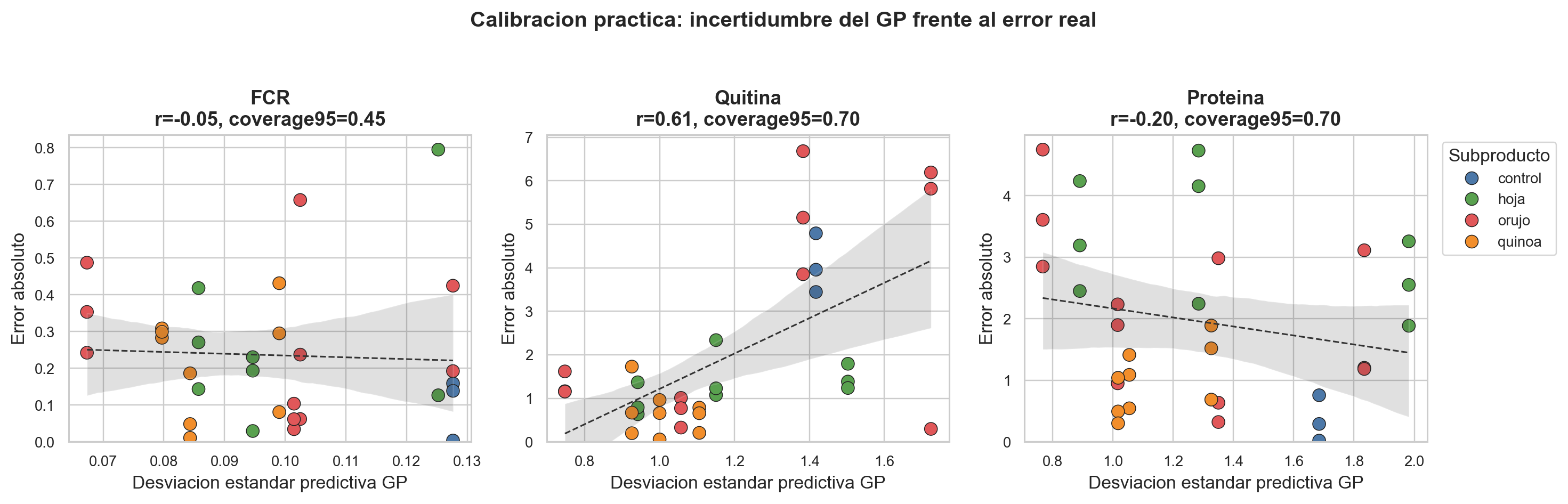
Consequently, the GP’s uncertainty is interpreted in this work as a supporting signal for decision-making, not as an absolute guarantee of reliability. Its role is especially useful for prioritizing future trials and detecting regions where the model acknowledges greater lack of knowledge. However, any candidate proposed from the surrogate must be understood as an experimental hypothesis pending validation, not as a closed conclusion about the actual performance of a new diet.

Prospective screening via EI

As a closing step for the real case, we analyze whether the trained GP can be used as a screening tool for a possible future experimentation phase. Unlike the benchmark experiment, here no physical infill cycle is executed: no new diets are tested and the dataset is not updated. The goal is solely to check whether the model allows prioritizing candidate formulations within a feasible space.

For this, EI is used, introduced in Section 2.4.3 and formulated earlier, adapting the orientation of each objective: FCR is minimized, while chitin and protein are maximized. The prospective space is built from the by-products considered in the real case, leaf, pomace, and quinoa, and from inclusion percentages within the observed range. Over this domain a grid is generated with $1\%$ increments, excluding formulations already tested.

Table 3.8 compares, for each objective, the best experimentally observed point with the untested candidate prioritized by EI.

Objective	Observed incumbent	EI candidate	Candidate prediction	EI	Reading
FCR	Quinoa30: $1.543$	Quinoa16	$1.726 \pm 0.065$	$2.7{\cdot}10^{-5}$	The predicted mean does not improve on the incumbent, so the candidate should be interpreted as exploratory.
Chitin	Orujo70: $15.318\%$	Orujo89	$12.658 \pm 1.061\%$	$0.002$	EI prioritizes a high-inclusion pomace region, although without surpassing on average the best observed value.
Protein	Orujo50: $32.147\%$	Orujo31	$30.938 \pm 0.912\%$	$0.038$	The candidate lies in an untested pomace zone, but the predicted mean remains below the incumbent.

Observed incumbents and prospective candidates prioritized by EI.

The results show that the EI candidates do not replace the best observed values: for FCR the incumbent remains Quinoa30, for chitin Orujo70, and for protein Orujo50. Furthermore, the candidates’ predicted means do not clearly surpass these incumbents. Therefore, the usefulness of EI in this case does not lie in demonstrating new optimal diets, but in turning the GP’s mean prediction and uncertainty into concrete proposals for a next experimental iteration.

Overall, this analysis should be interpreted as a pre-infill phase. The surrogate model reduces the search space and points to formulations with some informative value, but the final decision would require experimental validation. A complementary visualization of the EI landscape over the feasible grid is included in Annex 7.6.

Synthesis of results

Overall, the chapter’s results show a consistent reading across the two experimental scenarios. In the synthetic benchmarks, the GP + EI cycle improves the best value found relative to the initial design, especially when the model’s uncertainty helps direct new evaluations. In the real case, LODO validation indicates that the composite GP provides predictive capacity over the Dummy model on several objectives, although its uncertainty does not appear perfectly calibrated across all of them. Therefore, the surrogate model should not be interpreted as a tool capable of replacing experimental validation, but rather as a mechanism for reducing the search space, partially quantifying uncertainty, and proposing reasonable candidates for a next round of trials.

Conclusions and future work

The goal of this Bachelor’s Thesis (TFG) has been to address a decision-making problem: determining which new configurations are worth evaluating in a real experiment whose cost is high. As a starting point, an exhaustive study of the problem and the most suitable tools for solving it was carried out. All the knowledge developed has been presented rigorously and with sound foundations, starting from the principles of machine learning and delving into the theoretical bases of Bayesian processes, Bayesian optimization, and surrogate models. The purpose of this approach is not to replace the real experiment, but to leverage the information obtained from already-observed data to guide, more efficiently, the decisions about which next configurations are worth evaluating.

In a preliminary phase, synthetic experiments were carried out that allowed us to study, in a controlled environment, where the real function is known and where it is possible to check whether the search procedure improves on the initial design. In this scenario, the cycle formed by fitting the Gaussian process, selecting new points via Expected Improvement, and updating the observed set improved the best value found across all the benchmarks analyzed. This confirms that, when the model has a sufficient signal, it can guide the search toward more promising regions than those obtained solely from the initial design.

These preliminary experiments also show an important conclusion: a model that predicts well on average is not always the one that best helps with optimization. In this type of problem, it matters not only to reduce the average error but also to know how to use uncertainty to decide where it is worth exploring. Therefore, the usefulness of a Gaussian process does not depend solely on its predictive accuracy, but on its ability to combine prediction and uncertainty into a strategy for selecting new evaluations.

In the real case of diets for Hermetia illucens, the problem has been approached as a learning task based on already-available experimental data. To evaluate and validate the model in a way close to its practical use, a Leave-One-Diet-Out protocol was used, leaving out complete diets during training and checking whether the model is able to estimate their results. This approach is more demanding than predicting isolated replicates, given its similarity to the real case of wanting to assess a diet not yet tested.

Under this evaluation, the Gaussian process improves on the simple reference model for FCR, chitin, and protein. This indicates, therefore, that the diet’s formulation and composition variables contain useful information and that the model is not limited to merely memorizing the available data. Even so, the results should be interpreted with caution: the dataset is small, generalization is not equally good across all diets, and the predictive uncertainty appears only partially calibrated. Therefore, the model’s predictions should be understood as an aid for decision-making, not as a definitive biological conclusion.

An important reading of the real case is that the work sits at an early phase of the experimental cycle. With the current data, the model can propose candidate diets and point to regions that seem interesting, but it cannot yet confirm on its own which is the best formulation. Precisely for that reason, the infill process is relevant: by selecting new diets via a criterion such as Expected Improvement, testing them experimentally, and retraining the model with that new data, the Gaussian process could become progressively more robust, more useful for prioritizing candidates, and, potentially, better calibrated.

From an applied perspective, the recommendation for a scientific team working with feeds or diets would be to use this methodology as a support tool before designing the next round of trials. Rather than testing new formulations in an undirected way, the model allows leveraging already-conducted experiments to better rank the available options, identify promising candidates, and decide where it is most worth investing time and resources. Overall, the work shows that surrogate models do not replace experimental validation, but they can reduce the search space, quantify uncertainty, and help choose the next diets to test with more discernment.

Future work

The first line of future work consists of closing the experimental cycle of the real case. In this TFG, the real case reaches a pre-infill phase: the model is trained with the available data, validated via LODO, and used to propose prospective candidates. The natural next step would be to select one or several candidate formulations, test them experimentally, and retrain the GP with the new observations. In this way, the real case would move from a retrospective validation to a true sequential process of surrogate-based optimization.

A second line of continuation would be to formalize a multi-objective decision function. In the current analysis, FCR, chitin, and protein are studied separately, which allows each objective to be interpreted individually. However, from a production standpoint, choosing a diet usually depends on several simultaneous criteria, such as conversion efficiency, nutritional composition, cost, by-product availability, or experimental feasibility. Defining a decision rule together with expert judgment would allow studying trade-offs between objectives, not just individual optima.

It would also be important to expand the experimental dataset. The real case used contains 11 diets with 3 replicates per diet, sufficient for a first methodological validation but still limited for drawing strong biological conclusions. Incorporating new diets, more inclusion levels, and more replicates would improve the model’s stability, allow better study of uncertainty calibration, and check whether the learned relationships hold outside the currently observed range.

From a methodological standpoint, future extensions could explore models capable of handling several objectives jointly, such as multi-output Gaussian processes or hierarchical models. This would allow leveraging possible relationships between FCR, protein, and chitin, especially in low-data scenarios. It would also be interesting to study models with heteroscedastic noise or probabilistic recalibration techniques, given that the GP’s uncertainty does not behave the same across all objectives.

Lastly, the acquisition process could be extended beyond EI. Future versions could use multi-objective criteria, constrained criteria, or batch infill strategies that propose several diets to test in the same experimental round. These extensions would allow turning the developed framework into a more complete decision-support tool, capable of guiding successive experimental campaigns with more efficient use of the available budget.

Supplementary material for the benchmarks experiment

This appendix gathers the methodological and graphical material from the benchmarks experiment that has been removed from the main body to keep the report within the length limit. Chapter 3 retains the core elements of the analysis: the benchmarks table, the general experimental setup, the incumbent summary, the incumbent evolution, the predictive summary, and the hierarchy of experimental factors.

Detailed domain of the Borehole benchmark

Variable	Description	Domain
$r_w$	Borehole radius	$[0.05, 0.15]$
$r$	Radius of influence	$[100, 50000]$
$T_u$	Transmissivity of upper aquifer	$[63070, 115600]$
$H_u$	Upper piezometric head	$[990, 1110]$
$T_l$	Transmissivity of lower aquifer	$[63.1, 116]$
$H_l$	Lower piezometric head	$[700, 820]$
$L$	Borehole length	$[1120, 1680]$
$K_w$	Borehole hydraulic conductivity	$[9855, 12045]$

Domain of the Borehole benchmark.

Infill process flow

Infill process flow: initial design, GP training, mean and uncertainty prediction, EI computation and maximization, benchmark evaluation, data update, and result measurement. The cycle repeats until the budget is exhausted.

Detailed description of the infill process

The infill process reproduces an optimization scenario with costly evaluations, where each new point must be selected in an informed manner. In this experiment, the objective function is formulated as a minimization problem, so the expected improvement is calculated with respect to the best value observed so far.

At each iteration, the GP is fitted with the available set of observations $\mathcal{D}_n$ and the EI criterion is computed over the search domain. Although the objective function is minimized, EI is maximized, since the point with the greatest expected improvement is sought:

$$\bm{x}_{\mathrm{next}} = \operatorname*{arg\,max}_{\bm{x}\in\mathcal{X}} (EI(\bm{x})).$$

The maximization of EI is carried out via Differential Evolution, as this is a robust strategy for potentially multimodal acquisition functions and requires no gradients. In addition, polish=True is used, applying a local refinement with L-BFGS-B after the global search. Since SciPy’s optimizers are formulated as minimization problems, the implementation optimizes $-EI(\bm{x})$, which is equivalent to maximizing $EI(\bm{x})$.

Seed configuration and reproducibility

This section covers only the seed assignment used in the benchmark trajectories. The full computational configuration and the reproduction procedure are documented in Appendix 8.

Element	Seed used
Initial training	42
Test set	1042
Noise in training and test	42
Noise during infill	42
EI, Differential Evolution, and random fallback	At each iteration a step-dependent seed is used, $S + \text{step} \times 1009$, where $S$ is the configuration’s base seed.
Cross-validation audit in active mode	If the KFold audit is enabled, the seed depends on the step to preserve reproducibility of each iteration.

Seed configuration used in the benchmarks experiment.

Final improvement of the minimum found per benchmark

Figure 5.2 summarizes the optimization success of the infill process, not the overall predictive quality of the surrogate model. Branin shows the largest average reduction of the gap to the optimum, with GP_Matern52_ARD, followed by Forrester with GP_Matern52. Borehole also shows a strong improvement, although in this case the reduction of the best clean value is measured, since no reference optimum is available in the implementation. Hartmann6 shows a more moderate improvement with greater variability.

Overall, the figure confirms that EI enables finding better objective function values across all benchmarks, but it also shows that the magnitude of the improvement depends heavily on the problem. For this reason, the incumbent should be interpreted as the central metric of search success, complementary to MAE and the rest of the predictive metrics.

Relative evolution of MAE

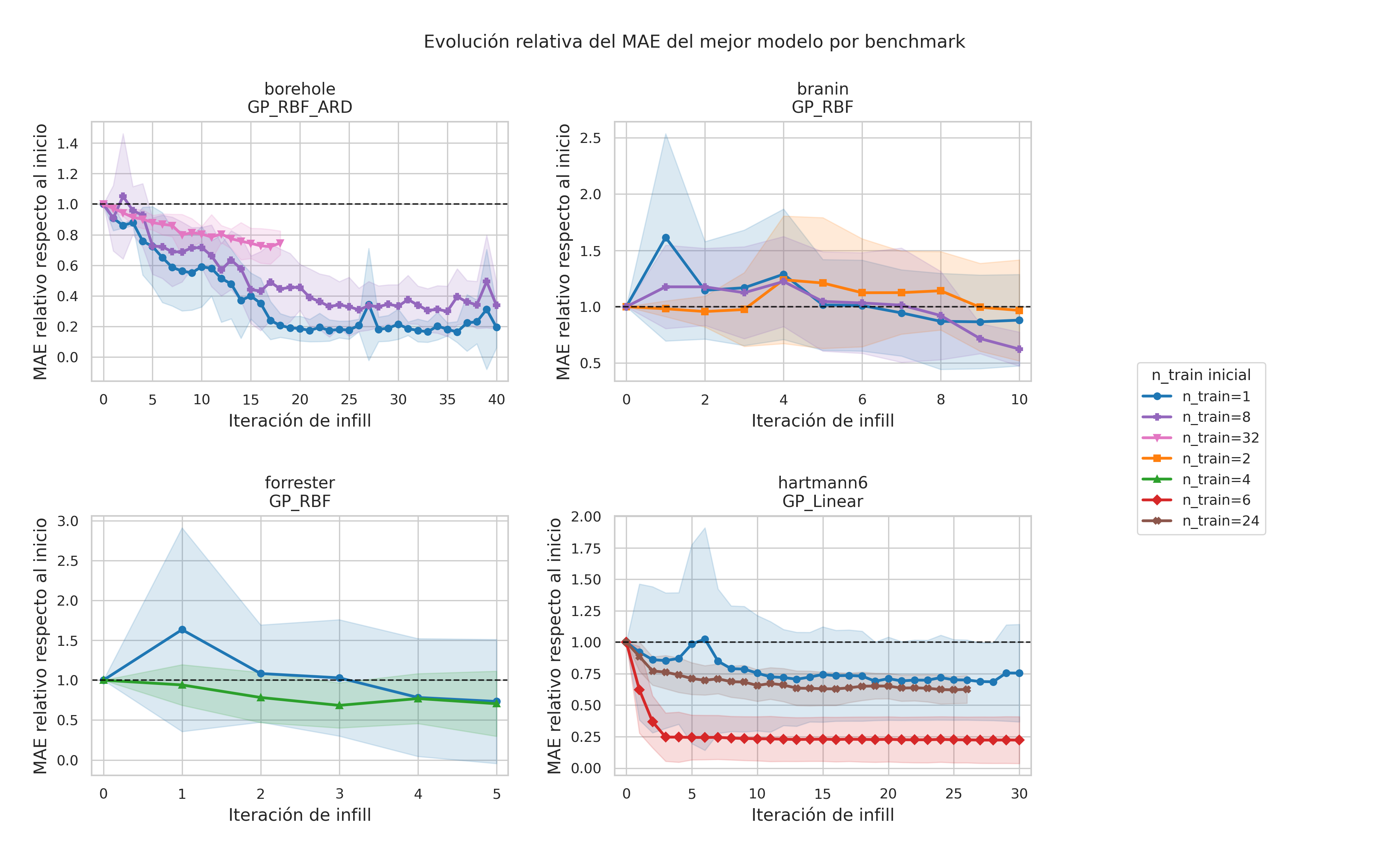
Figure 5.3 shows the evolution of the relative MAE during the infill process for the best predictive model of each benchmark. The dashed line at $1$ represents the error of the model trained only with the initial design; therefore, values below $1$ indicate a reduction in MAE and values above reflect a temporary worsening.

The clearest pattern appears in Borehole, where GP_RBF_ARD reduces the error steadily, especially when the initial design is small. In Hartmann6 a rapid improvement is also observed, particularly for $n_{\mathrm{train}}=6$, where GP_Linear achieves a marked reduction in MAE. In contrast, Branin and Forrester show less monotonic trajectories: some configurations worsen initially before stabilizing or improving. This indicates that adding points via EI does not always immediately reduce the overall error.

Overall, the figure shows that infill can improve the predictive quality of the surrogate model, but that this improvement depends on the benchmark, the initial size, and the model. Furthermore, relative MAE should not be confused with optimization success: EI selects points to improve the search for the optimum, not necessarily to monotonically minimize the predictive error across the whole domain.

Predictive and probabilistic diagnostics

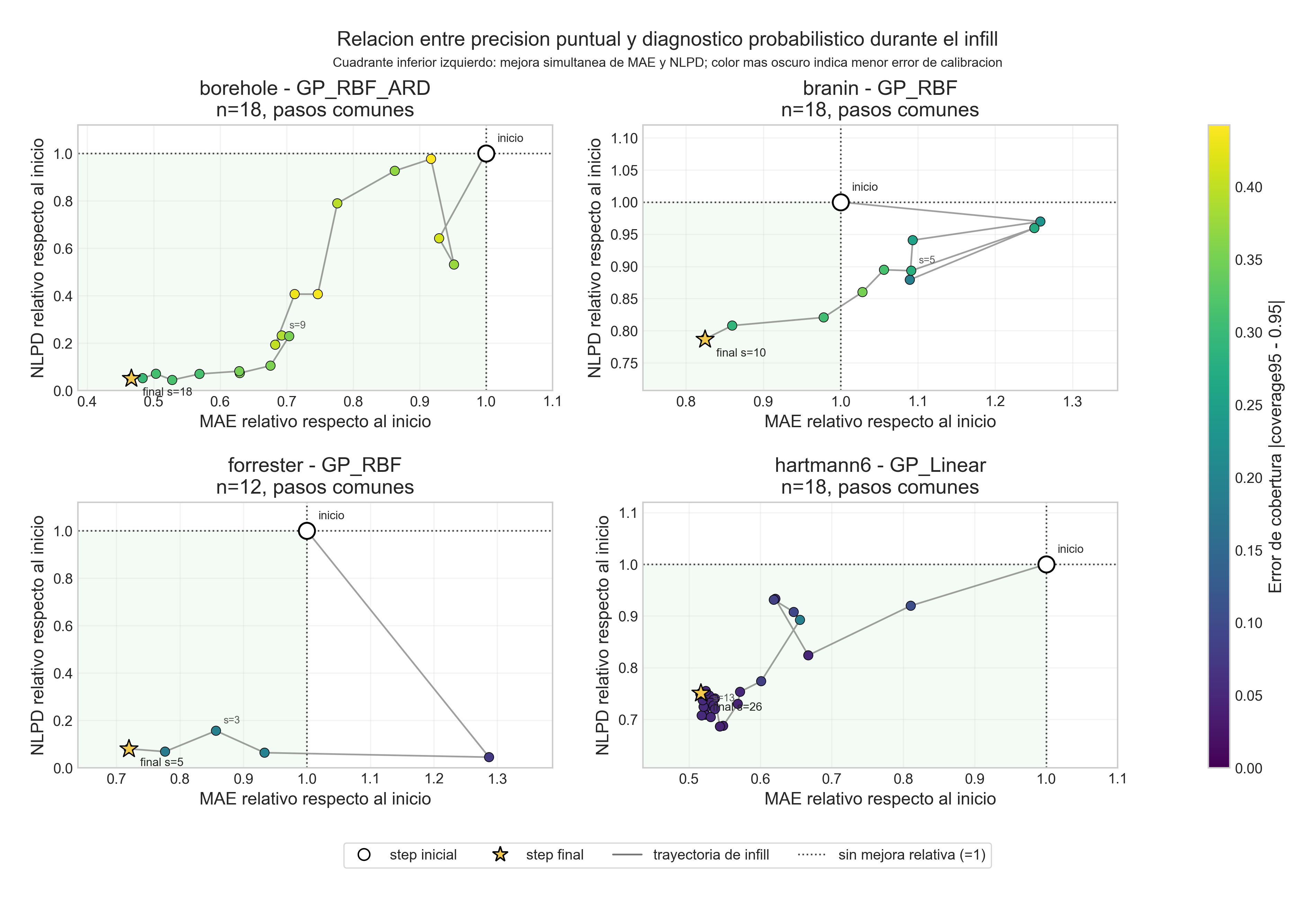
Figure 5.4 relates the improvement in pointwise error to the improvement in probabilistic diagnostics during infill. The horizontal axis shows the relative MAE and the vertical axis the relative NLPD, both with respect to the start. Therefore, the lower-left quadrant represents the desirable case: lower mean error and better probabilistic quality than in the initial design. Color adds a third reading, the calibration error of $95\,\%$ coverage, where darker tones indicate better-calibrated intervals.

All four benchmarks end up in the zone of simultaneous improvement, though with nuances. Borehole shows the clearest improvement in MAE and NLPD, with a final point close to $0.47$ in relative MAE and $0.05$ in relative NLPD; however, it maintains undercoverage, so the uncertainty is not fully calibrated. Forrester also improves markedly in NLPD and moderately in MAE. Branin shows a smoother improvement and a less direct trajectory. Hartmann6 offers the most balanced behavior: it reduces MAE while maintaining calibration close to $95\,\%$.

The main conclusion is that predictive improvement should not be evaluated using MAE alone. A model can reduce the mean error while still providing poorly calibrated uncertainty intervals. Therefore, this figure complements the MAE evolution and justifies jointly analyzing pointwise accuracy, NLPD, and predictive coverage.

Effect of experimental conditions

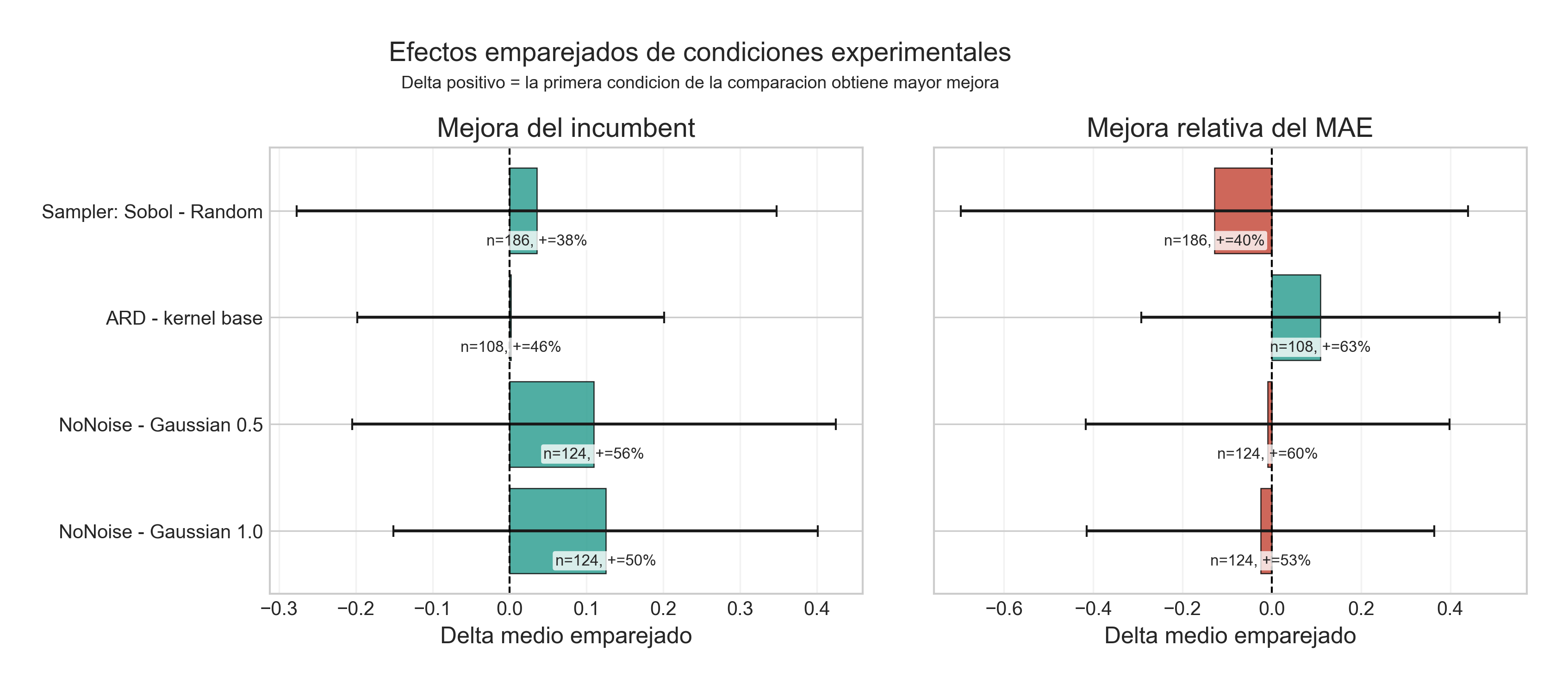
Figure 5.5 compares the average effect of different experimental conditions while keeping the remaining configurations paired. The deltas are, in general, small relative to their variability, indicating that no single factor consistently dominates the outcome. In terms of incumbent improvement, the absence of noise shows a moderate positive effect compared to Gaussian noise, while Sobol versus random and ARD versus base kernel show weak effects.

For MAE, ARD tends to slightly improve the average result, but with high dispersion. Sobol sampling shows no clear advantage over random sampling, and the effect of noise on MAE is small. Therefore, the figure suggests that the final behavior depends more on the benchmark and the interaction between conditions than on any single isolated experimental decision.

Supplementary analysis of the infill process

This appendix complements the benchmark material of Appendix 5 with a visual and statistical reading of the infill process. The goal is not to introduce new main results, but to show in more detail how the surrogate model participates in the sequential selection of points and why predictive metrics and optimization metrics do not always select the same model.

Relationship between predictive improvement and improvement of the minimum found

Table 6.1 compares, for each benchmark, the model with the greatest improvement in the minimum found against the model with the greatest relative improvement in MAE. This comparison is relevant because the goal of an infill optimization cycle is not necessarily to minimize the global mean error of the surrogate model, but to find better values of the objective function with a limited budget of evaluations.

Benchmark	Best model by minimum found	Improvement inc.	Best model by MAE	MAE improvement
Borehole	GP_Linear	0.720	GP_RBF_ARD	0.574
Branin	GP_Matern52_ARD	0.898	GP_RBF	0.175
Forrester	GP_Matern52	0.737	GP_RBF	0.281
Hartmann6	GP_RBF	0.434	GP_Linear	0.466

Comparison between the best model according to improvement of the minimum found and the best model according to relative MAE improvement.

In all the benchmarks in Table 6.1, the model that most reduces the mean error does not necessarily coincide with the model that achieves the greatest improvement in the minimum found. This result justifies analyzing separately the predictive quality of the surrogate model and the effectiveness of the search process.

Forrester as a visual case of the infill mechanism

Forrester is used as a visual case because it is a one-dimensional benchmark. This property allows simultaneously representing the real function, the posterior mean of the GP, the predictive uncertainty, and the observed points. It is therefore well suited to graphically explain the role of EI in the selection of new evaluations.

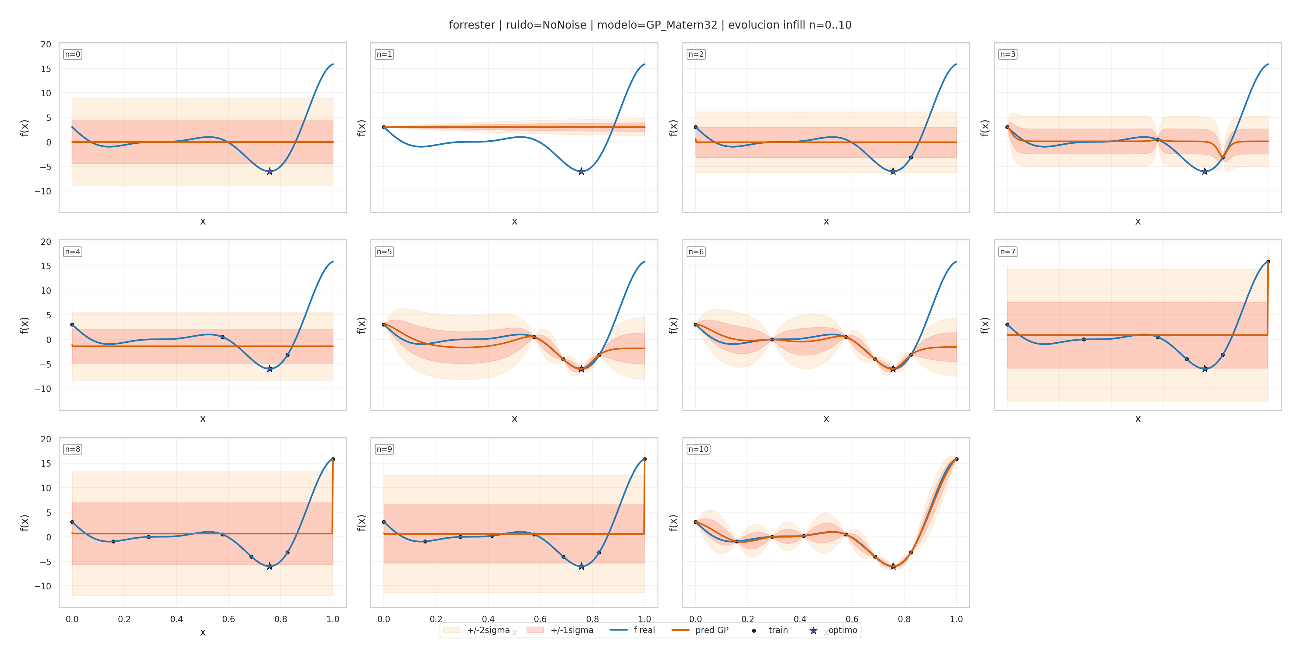
Figure 6.1 allows us to observe how the surrogate model changes as new observations are incorporated. In the early iterations, uncertainty dominates large areas of the domain. As the process progresses, the model better fits the region near the minimum and reduces uncertainty around the evaluated points. This visualization helps interpret why the process should not be evaluated solely through MAE: an imperfect global prediction can still be useful if it guides the search toward promising regions.

Point decision through Expected Improvement

Figure 6.2 shows a specific EI decision in Forrester. The GP is trained with four initial Sobol points and several previous infill evaluations. In the step shown, EI proposes the next point at $x_{\mathrm{next}}=0.763$, very close to the known optimum of the benchmark.

Element	Value
Benchmark	Forrester
Model	GP_Matern52
Initial design	Sobol, $n_{\mathrm{train}}=4$, no noise
Infill step	5
Proposed point	$x_{\mathrm{next}}=0.763$
EI at the proposed point	1.519
Best value observed before	-4.364
Value observed at $x_{\mathrm{next}}$	-6.004
Known optimum	$f(x^\star)=-6.021$
Gap closed after evaluation	99.0 %

Numerical summary of the EI decision represented in Figure 6.2.

This example shows the practical role of uncertainty in a GP. EI does not select a new point solely based on the predicted mean, but on the combination of expected improvement and predictive dispersion. In this case, the chosen point ends up very close to the real optimum and reduces almost entirely the gap that existed before the evaluation.

Complementary statistical contrasts

In addition to the descriptive tables, the records generated by the experiment allow performing nonparametric tests on the benchmark results. These tests are not intended as a formal demonstration of universal superiority, but as a complementary check of two effects observed in the main analysis: the improvement of the incumbent during the infill process and the existence of differences between GP kernel families.

To evaluate the improvement of the incumbent, the best value observed at the beginning and at the end of each active trajectory was compared. Each trajectory is defined by benchmark, sampler, initial size, noise configuration, validation mode, and model. Since the benchmark objective function is formulated as minimization, a reduction in the incumbent indicates improvement. Table 6.3 summarizes a one-sided Wilcoxon signed-rank test, with the alternative of improvement after the infill process.

Model	Trajectories	Improve	Median improvement	$p$-value
All GPs	372	316	2.812	$7.35\times10^{-54}$
GP_Linear	66	30	0.000	$8.67\times10^{-7}$
GP_Matern32	66	62	2.970	$3.79\times10^{-12}$
GP_Matern52	66	60	2.519	$8.15\times10^{-12}$
GP_Matern52_ARD	54	54	8.105	$8.13\times10^{-11}$
GP_RBF	66	59	2.574	$1.20\times10^{-11}$
GP_RBF_ARD	54	51	7.602	$2.57\times10^{-10}$

Contrast of incumbent improvement between the start and end of the infill trajectories.

The results show that the infill process systematically reduces the incumbent in the trajectories considered. The effect is especially clear in the ARD kernels and in the Matérn/RBF kernels, while the linear model shows a null median improvement, although without worsening in many configurations and with occasional improvements sufficient for the aggregate test to be significant.

To compare GP kernels in predictive terms, the MAE of the complete blocks shared by all kernels was used. Each block corresponds to a combination of benchmark, sampler, initial size, noise configuration, and validation mode. Over the 54 complete blocks, the Friedman test detects differences between models $(p=1.88\times10^{-6})$. Table 6.4 shows the mean ranks and the pairwise Wilcoxon contrasts against the kernel with the best mean rank.

Model	Mean rank	$p$ vs. GP_Matern52_ARD	Reading
GP_Matern52_ARD	2.741	—	Best mean rank.
GP_RBF_ARD	2.815	0.677	Practically indistinguishable performance from the best.
GP_Matern52	3.370	$4.51\times10^{-4}$	Worse than the ARD version in the pairwise contrast.
GP_RBF	3.593	0.138	Inconclusive difference compared to the best.
GP_Matern32	4.056	$2.04\times10^{-5}$	Worse than the best kernel on the shared blocks.
GP_Linear	4.426	$5.28\times10^{-8}$	Lower aggregate predictive performance.

Nonparametric comparison between GP kernels using MAE on complete blocks. Lower ranks indicate better behavior.

These contrasts support two conclusions used in the report: first, the infill cycle provides an effective improvement over the best observed value; second, ARD kernels tend to occupy the best positions in MAE. However, no clear statistical separation is observed between GP_Matern52_ARD and GP_RBF_ARD, so the choice of a specific kernel should be interpreted together with stability, computational cost, and behavior on each problem.

Supplementary material for the real case

This appendix collects supporting material from the real Hermetia illucens case. Its purpose is to document the traceability of the modeled dataset and to provide complementary figures that help interpret the results of Chapter 3, without replacing the main figures on LODO generalization, kernel comparison, uncertainty, and pre-infill.

Inventory of generated datasets

The preparation pipeline generates several datasets from the original experimental files. However, the modeling of the real case is limited to the Hermetia productivity dataset, for the reasons of scope and homogeneity described in Chapter 3. Table 7.1 summarizes the datasets generated and their role in the work.

Dataset	Rows	Diets	Species	Use
productivity_hermetia_lote.csv	33	11	Hermetia	Dataset modeled in the real case preparation pipeline.
productivity_tenebrio_lote.csv	57	19	Tenebrio	Dataset generated and available, not modeled in the current results.
productivity_all_lote.csv	90	19	Both	Combined dataset available for subsequent analyses.
quality_hermetia_dieta.csv	11	11	Hermetia	Diet quality dataset generated as support material.
quality_tenebrio_dieta.csv	19	19	Tenebrio	Diet quality dataset generated as support material.
quality_all_dieta.csv	30	19	Both	Combined quality dataset available.

Inventory of datasets generated in the Entomotive case.

In the modeled dataset, the 33 observations correspond to 11 diets with three replicates per diet. The targets used are FCR, QUITINA (%), and PROTEINA (%). Availability is complete for chitin and protein, with 33 valid values, and slightly lower for FCR, with 31 valid values.

Observed values by diet

Figure 7.1 summarizes the mean observed values per diet for the three targets of the real case. This figure is not used as a main model result, but as a prior descriptive check: it allows us to see that the best observed values do not always belong to the same diet, and that the problem has a multiobjective nature.

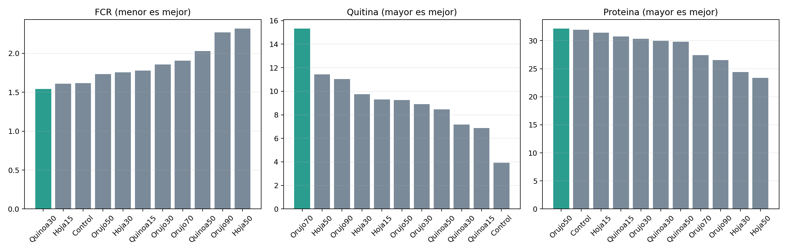
Target	Criterion	Diet	Byproduct	Mean observed value
FCR	Minimize	Quinoa30	quinoa	1.543
Chitin	Maximize	Orujo70	pomace	15.318
Protein	Maximize	Orujo50	pomace	32.147

Best observed diets by individual target.

Parity of the best GP per target

Figure 7.2 complements the aggregate metrics from Chapter 3. Instead of summarizing error into a single value, it plots observed versus predicted values in LODO validation for the best GP of each target. The diagonal line indicates perfect prediction.

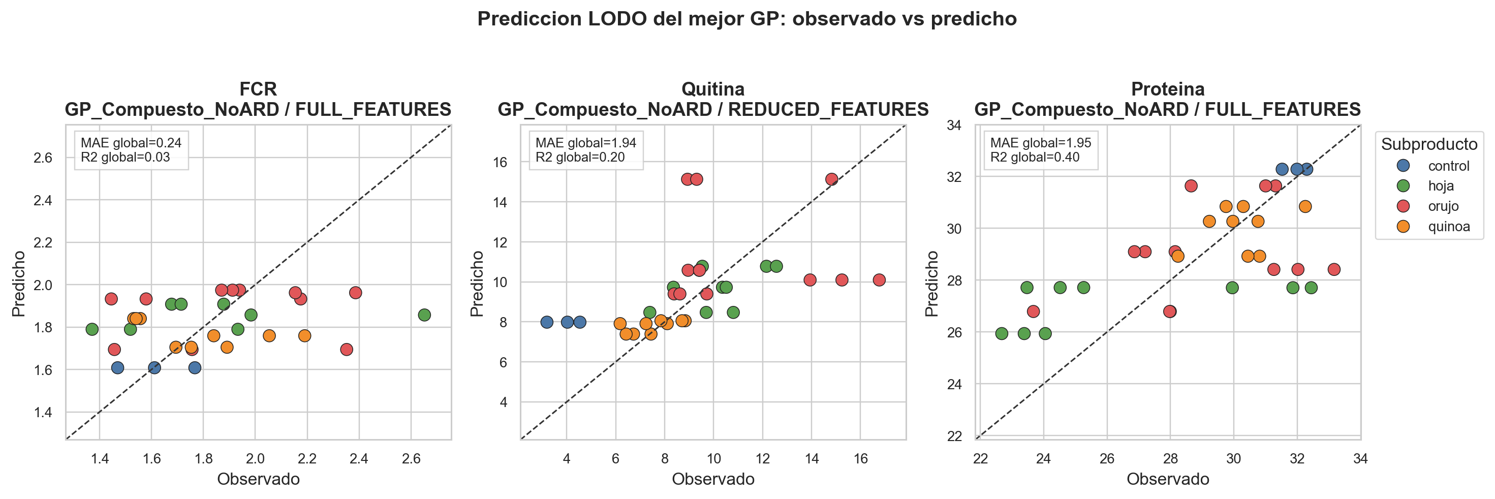
This figure allows us to detect patterns that remain hidden in the macro MAE. For FCR, predictions tend to concentrate within a narrow range, which indicates difficulty extrapolating between diets. For chitin and protein, a clearer signal is observed, although with relevant errors for some byproducts. Therefore, the model provides useful information, but should not be interpreted as a substitute for the experimental trial.

LODO contrasts against the Dummy baseline model

The LODO results for the real case also allow for a complementary statistical reading, although necessarily cautious given the sample size. In this analysis, each diet held out in LODO validation is used as a paired unit, so that the models are compared over the same training and test partitions. The metric used is the MAE per diet, since it is the main metric of the generalization analysis.

A Friedman test was first applied per target to compare all available models. Then, as a directed contrast against the baseline model, a one-sided Wilcoxon signed-rank test was applied between the Dummy and the GP with the best mean rank for each target. The $p$-values should be interpreted as exploratory evidence, not as conclusive proof, because each target has only 11 diets available.

Target	Reference GP	Rank	$p_F$	Improvement	$\Delta$MAE med.	Reading
FCR	GP_Matern32_NoARD	3.455	0.521	8/11	0.017	Favorable trend for the GP, but no conclusive evidence against the Dummy $(p=0.062)$.
Protein	GP_Matern32_ARD	3.273	0.209	9/11	0.827	Favorable evidence for the GP against the Dummy $(p=0.034)$; other GP kernels also show exploratory significant improvements.
Chitin	GP_Linear	2.636	0.194	8/11	0.380	Positive median improvement, but non-conclusive contrast $(p=0.160)$.

Complementary contrasts on the per-diet LODO MAE against the Dummy baseline model. \DeltaMAE represents MAE_{\mathrm{Dummy}}-MAE_{\mathrm{GP}}, so positive values favor the GP.

The main reading of these contrasts is consistent with the parity figures and the aggregate metrics. For protein, the GP model provides a more consistent improvement over the baseline model. For FCR, a weak signal is observed, consistent with the difficulty of extrapolating between diets and with the concentration of predictions within a narrow range. For chitin, although some folds favor the GP, the evidence is not sufficient to claim a statistically robust improvement with the available data.

Predictive intervals by diet

Figure 7.3 shows, for each diet held out in LODO validation, the predictive mean of the GP together with approximate $95\,\%$ intervals. This visualization complements the calibration analysis presented in Section 3.3.6.3, since it allows us to observe, in a disaggregated way, in which diets the intervals reasonably contain the observed values and in which specific coverage failures appear.

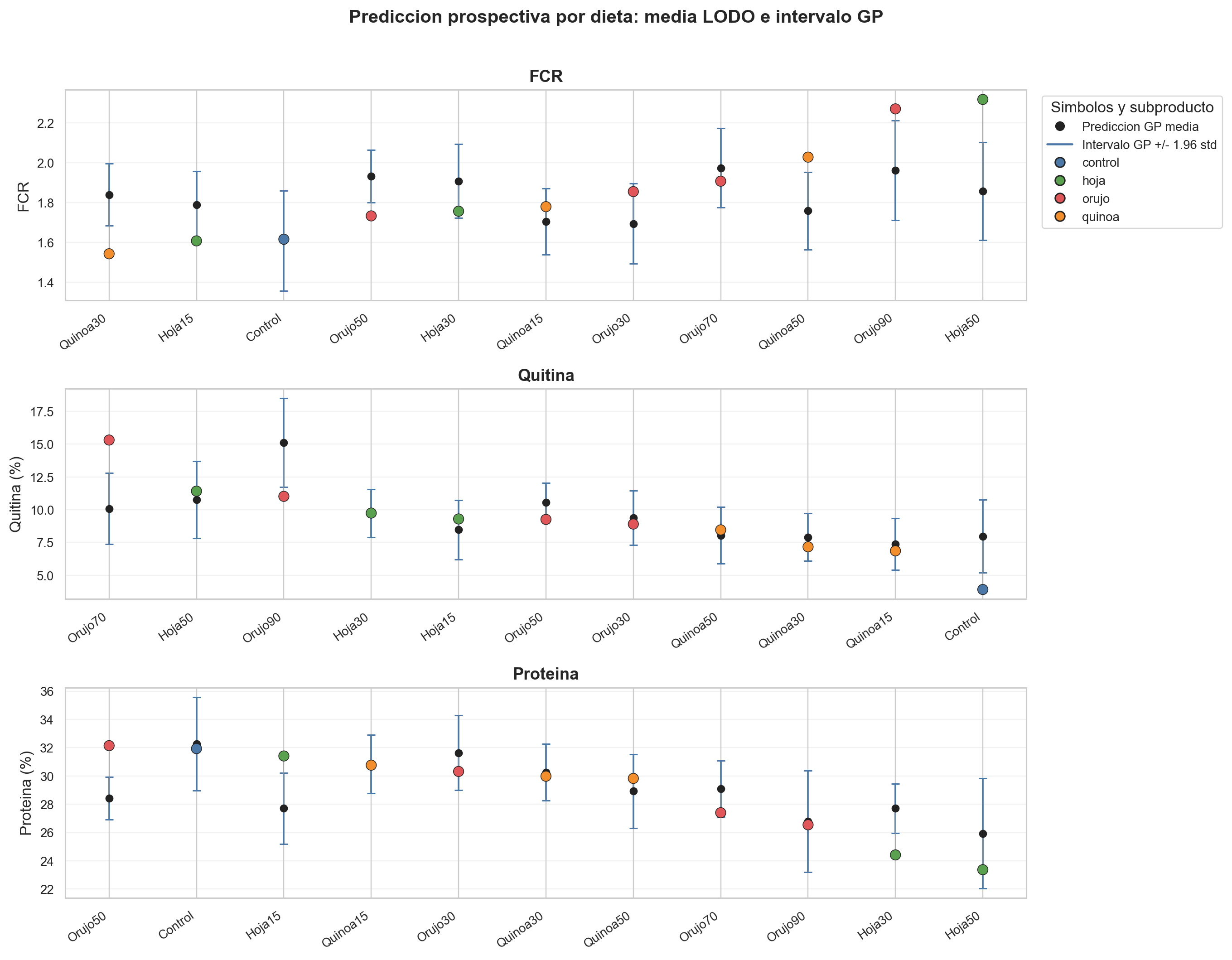
Prospective EI landscape

Figure 7.4 shows the prospective EI landscape over the feasible grid of formulations considered in the real case. This visualization complements the screening presented in Section 3.3.6.4, where the observed incumbents are compared against untested candidates prioritized by EI.

The purpose of this figure is not to demonstrate that the proposed candidates are optimal, but to show how the acquisition criterion distributes prospective value across the search space. Areas with higher EI correspond to combinations in which the model identifies a possible improvement over the observed state or an uncertainty relevant enough to justify a future evaluation.

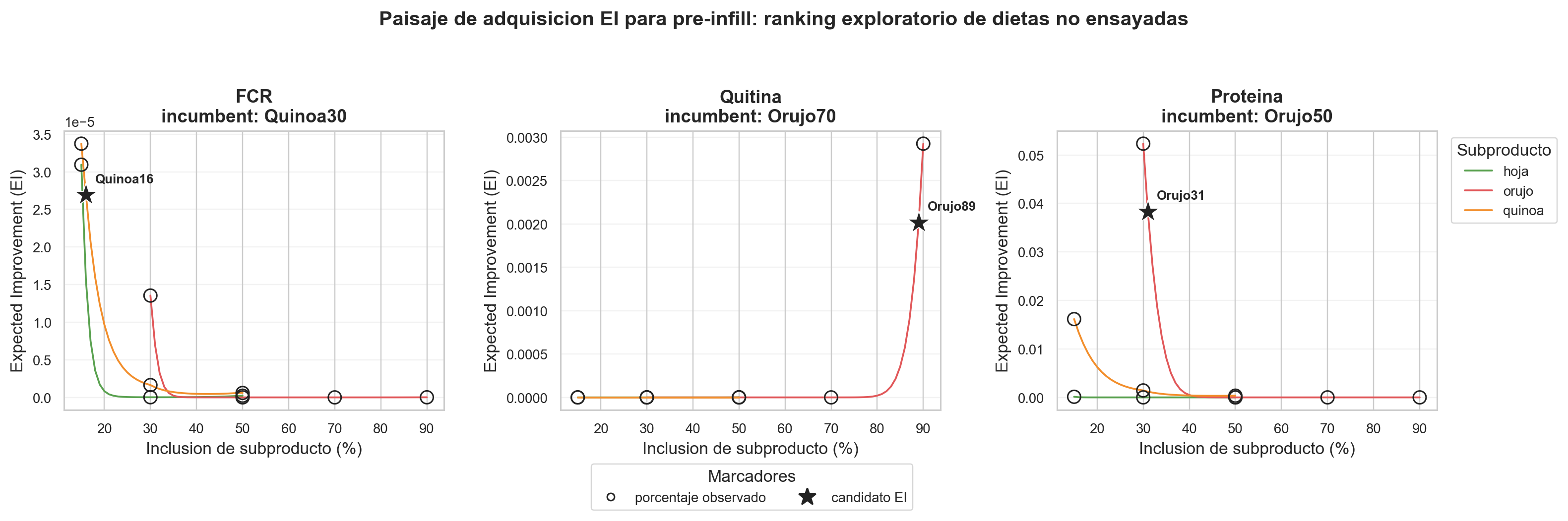
Therefore, this figure should be interpreted as a support tool for subsequent experimental design. In the current state of the work, the points highlighted by EI constitute testing hypotheses, not validated experimental results.

Computational configuration and reproducibility

This appendix documents the computational configuration used to generate the results of the work. Its aim is not to introduce new methodology, but to leave traceable how the experimental protocol, the code, and the output files used in the report are connected. Unlike Appendices A—C, which focus on results and supplementary figures, here only the configuration needed to reproduce them is collected.

Benchmark experiment configuration

The benchmark experiment reproduces an optimization scenario with limited evaluations. For each function, an initial design is generated, a GP is fitted, and new observations are added via EI. The relevant configuration comes from src/configs/benchmark_tuning_specs.py and the active learning logic implemented in src/analysis/active_learning.py. Table 8.1 summarizes the values used.

Element	Configuration
Benchmarks retained in the report	Forrester, Branin, Hartmann6, and Borehole.
Initial sampling	Sobol and uniform random sampling.
Initial sizes	$n_{\mathrm{train}}\in\{1,d,4d\}$, where $d$ is the dimension of the benchmark.
Test set	200 points generated within the domain of each benchmark.
Synthetic noise	No noise, Gaussian noise with $\sigma=0.5$, and Gaussian noise with $\sigma=1.0$.
Model families	Dummy, linear GP, RBF GP, Matérn $3/2$ GP, Matérn $5/2$ GP; for dimension greater than one, ARD variants are included in RBF and Matérn $5/2$.
Infill budget	$5d$ new evaluations, with a maximum of 50 total observations during the trajectory.
Acquisition function	Expected Improvement with exploration parameter $\xi=0.01$.
EI optimization	Differential Evolution over the continuous domain of the benchmark, with subsequent local refinement. In the implementation, $-EI(\bm{x})$ is minimized, which is equivalent to maximizing $EI(\bm{x})$.
EI optimizer budget	$\max(2000,500d)$ equivalent candidate evaluations to size the acquisition search.
Base seed	42. At each infill step, the EI seed shifts as $42 + 1009\cdot \mathrm{step}$.

Computational configuration of the benchmark experiment.

The noise levels used are absolute and therefore do not represent the same relative severity across all benchmarks. For this reason, the noise analysis should be understood as a robustness test of the pipeline under fixed perturbations, not as a normalized comparison of the effect of noise across functions.

The internal GP hyperparameters, such as characteristic lengths, signal amplitude, and white noise level, are re-estimated during the fitting of the GaussianProcessRegressor through maximization of the marginal log-likelihood. Therefore, in the benchmarks, each kernel family should not be interpreted as a fixed set of numerical parameters, but as a structural covariance hypothesis that is fitted to the data available at each iteration.

The implementation also contains benchmark-specific grids in benchmark_grids.py. These grids serve as support for audits or tuning modes, but the main reading of the report focuses on the aggregate comparison of GP families, the effect of the initial design, noise, the sampling method, and the evolution of the incumbent during the infill process.

Real case configuration

The real case is executed from the productivity_hermetia_lote.csv dataset. For each objective, an input matrix, a response vector, and a vector of groups by diet are constructed. The validation group is not the replicate, but the complete diet, so that the three replicates of a formulation remain together in training or in test.

Three active objectives are evaluated: FCR, chitin, and protein. FCR is interpreted as a variable to minimize, while chitin and protein are interpreted as variables to maximize in the prospective phase. The final availability is 31 observations for FCR and 33 observations for chitin and protein.

Input representations

Two input representations are compared. Both include numerical variables of formulation and diet composition, along with binary indicators of the by-product type. The diet name is used to define the LODO groups, but it is not used as a direct predictor variable.

Mode	Dimension	Variables included
Reduced	9 variables	Five numerical variables: inclusion percentage, mean diet protein, mean fiber, mean fat, and mean TPC of the diet. Four binary by-product indicators are added to these: control, leaf, pomace, and quinoa.
Full	14 variables	The variables of the reduced mode, plus mean ash, mean carbohydrates, and three derived ratios: protein/carbohydrates, protein/fiber, and fiber/fat. It also includes the four by-product indicators.

Input representations used in the real case.

The selected input variables do not present missing values in the final dataset used. Median imputation exists in the preparation flow as a safety mechanism, but it does not modify the input representation in the main results. Variable scaling is performed within the model’s Pipeline, so the standardization parameters are fitted only with the training of each fold.

Models and grids of the real case

The fitting of the real case uses nested LODO validation. In each outer fold, a complete diet is held out as test. On the remaining diets, an internal LODO validation is run to select hyperparameters. Then, the model is retrained with all the diets from the outer training set and evaluated on the held-out diet. The internal selection metric is MAE.

Model	Description
Dummy	Constant baseline. The grid allows selecting between the mean and median of the internal training set.
Linear GP	DotProduct kernel plus white noise. Represents a global linear trend.
RBF GP	RBF kernel plus white noise. Evaluated in isotropic version and, where applicable, with ARD.
Matérn $3/2$ GP	Matérn kernel with $\nu=3/2$ plus white noise. Evaluated in isotropic version and, where applicable, with ARD.
Matérn $5/2$ GP	Matérn kernel with $\nu=5/2$ plus white noise. Evaluated in isotropic version and, where applicable, with ARD.
Composite GP	Sum of a linear component, a Matérn $5/2$ component, and white noise. In the final protocol it is evaluated without ARD to avoid excessive exploration of variants on a small dataset.

Model families evaluated in the real case.

The common GP grid is summarized in Table 8.4. Each kernel family is evaluated with the structure indicated in Table 8.3. Within each fold, GaussianProcessRegressor optimizes the continuous kernel parameters through the marginal log-likelihood.

Parameter	Values considered
alpha	$\{10^{-10},10^{-5},10^{-2},1.0\}$. This term is added to the diagonal of the kernel matrix during fitting and helps control numerical stability and effective regularization.
kernel	One kernel structure per model family: linear, RBF, Matérn $3/2$, Matérn $5/2$, or composite.
normalize_y	True. The target variable is normalized internally during the GP fitting.
n_restarts_optimizer	15 restarts of the marginal log-likelihood optimizer.
White noise	WhiteKernel with initial level $10^{-4}$ and bounds $[10^{-7},0.8]$.
Characteristic lengths	In isotropic kernels a common initial scale is used. In ARD an initial vector of ones is used, with one scale per input variable. The bounds are $[10^{-2},10^{5}]$.

Hyperparameter grid used in the real case.

To limit the number of models on a small dataset, ARD is not applied to all families indiscriminately. First the base families are compared and then an ARD variant selected by combination of objective and input representation is evaluated. Table 8.5 summarizes those variants.

Representation	Objective	ARD variant evaluated
Reduced	FCR	RBF GP ARD
Reduced	Chitin	RBF GP ARD
Reduced	Protein	Matérn $3/2$ GP ARD
Full	FCR	Matérn $5/2$ GP ARD
Full	Chitin	Matérn $5/2$ GP ARD
Full	Protein	Matérn $3/2$ GP ARD

ARD variants evaluated by combination of objective and representation.

Prevention of information leakage

The prevention of information leakage is especially relevant in the real case, because the observations are diet replicates and not independent samples without structure. The protocol prevents leakage through four decisions:

1. Grouping by diet. All replicates of the same formulation share the same group. In each outer fold, a complete diet is left out.

2. Nested selection. The diet held out in the outer fold does not participate in hyperparameter selection. Selection is performed with internal LODO on the training diets.

3. Scaling within the model. The standardization of $X$ is fitted within the Pipeline using only the training data of the corresponding fold.

4. Structural use of the by-product type. The model receives by-product indicators and composition variables, but does not use the diet name as a direct predictive identifier. The diet name is reserved for building the LODO groups.

The binary encoding of the by-product type is constructed from an experimental variable known beforehand. This encoding does not use the response of the held-out fold. Consequently, the main leakage risk that is avoided is not knowing which by-products exist, but allowing replicates of a diet to appear simultaneously in training and test.

Reproduction of real case results

The real case can be reproduced with the reproduce_tfg_outputs.py script. By default, this script reuses the already computed fitting records, runs the audit, regenerates the final figures, and copies the necessary graphic resources to the thesis’s resources folder. If a complete recalculation of the LODO fitting is desired, it can be run with the --rerun-tuning option.

python reproduce_tfg_outputs.py
python reproduce_tfg_outputs.py --rerun-tuning

The script checks that the expected results exist for the two input representations and the three active objectives. In the recorded run, the reproducibility manifest collects 6 fitting summaries and 42 fold files, corresponding to the combinations of representation, objective, and active models. The manifest file is saved at:

outputs/reproducibility_real_case_manifest.json

The reproducibility documented in this appendix has two levels. First, the real case can be regenerated from the existing fitting records, which allows reconstructing the tables, audits, figures, and graphic resources used by the report. Second, if the complete fitting is run, the nested LODO models are recalculated from the Hermetia dataset. This second option is computationally more costly because it repeats the internal hyperparameter selection for each outer fold, objective, representation, and model family.

In the benchmarks, the results depend on the seeds, the sampling method, the initial size, the noise, and the infill budget. For this reason, the report does not interpret individual trajectories as definitive conclusions, but rather aggregate patterns across the evaluated configurations. This distinction is important: the goal of the benchmark experiment is to study the behavior of the GP + EI cycle under controlled conditions, while the goal of the real case is to check whether the same framework can provide useful signal before proposing a new experimental campaign.

Acronyms

GP	Gaussian Process
BO	Bayesian Optimization
SBO	Surrogate-Based Optimization
DoE	Design of Experiments
BB	Black-Box
RMSE	Root Mean Squared Error
MAE	Mean Absolute Error
NLL	Negative Log-Likelihood
LHS	Latin Hypercube Sampling
CV	Cross-Validation
ARD	Automatic Relevance Determination
RBF	Radial Basis Function
SE	Squared Exponential (also RBF)
LML	Log Marginal Likelihood (marginal log-likelihood / evidence)
EI	Expected Improvement
DE	Differential Evolution

References

Bishop, Christopher M. 2006. Pattern Recognition and Machine Learning. Information Science and Statistics. Springer.

Dixon, L. C. W., and G. P. Szegö. 1978. “The Global Optimization Problem: An Introduction.” In Towards Global Optimisation 2, edited by L. C. W. Dixon and G. P. Szegö. North-Holland.

Forrester, Alexander I. J., András Sóbester, and Andy J. Keane. 2008. Engineering Design via Surrogate Modelling: A Practical Guide. Wiley. https://doi.org/10.1002/9780470770801.

Gneiting, Tilmann, and Adrian E. Raftery. 2007. “Strictly Proper Scoring Rules, Prediction, and Estimation.” Journal of the American Statistical Association 102 (477): 359—78. https://doi.org/10.1198/016214506000001437.

Hastie, Trevor, Robert Tibshirani, and Jerome Friedman. 2009. The Elements of Statistical Learning: Data Mining, Inference, and Prediction. 2nd ed. Springer Series in Statistics. Springer. https://doi.org/10.1007/978-0-387-84858-7.

Jiang, Ping, Qi Zhou, and Xinyu Shao. 2020. Surrogate Model-Based Engineering Design and Optimization. Springer Tracts in Mechanical Engineering. Springer Singapore. https://doi.org/10.1007/978-981-15-0731-1.

Jones, Donald R., Matthias Schonlau, and William J. Welch. 1998. “Efficient Global Optimization of Expensive Black-Box Functions.” Journal of Global Optimization 13 (4): 455—92. https://doi.org/10.1023/A:1008306431147.

Kuleshov, Volodymyr, Nathan Fenner, and Stefano Ermon. 2018. “Accurate Uncertainties for Deep Learning Using Calibrated Regression.” Proceedings of the 35th International Conference on Machine Learning, Proceedings of machine learning research, vol. 80: 2796—804. https://proceedings.mlr.press/v80/kuleshov18a.html.

Morris, Max D., Toby J. Mitchell, and Donald Ylvisaker. 1993. “Bayesian Design and Analysis of Computer Experiments: Use of Derivatives in Surface Prediction.” Technometrics 35 (3): 243—55. https://doi.org/10.1080/00401706.1993.10485320.

NIST Digital Library of Mathematical Functions. 2010. “Chapter 10: Bessel Functions.” Edited by Frank W. J. Olver, Daniel W. Lozier, Ronald F. Boisvert, and Charles W. Clark. https://dlmf.nist.gov/10.

Rasmussen, Carl Edward, and Christopher K. I. Williams. 2006. Gaussian Processes for Machine Learning. Adaptive Computation and Machine Learning. MIT Press. http://www.GaussianProcess.org/gpml.

Schölkopf, Bernhard, Ralf Herbrich, and Alexander J. Smola. 2001. “A Generalized Representer Theorem.” Computational Learning Theory, Lecture notes in computer science, vol. 2111: 416—26. https://doi.org/10.1007/3-540-44581-1_27.

Settles, Burr. 2009. Active Learning Literature Survey. Computer Sciences Technical Report No. 1648. University of Wisconsin—Madison.

Sobol’, Ilya M. 1967. “On the Distribution of Points in a Cube and the Approximate Evaluation of Integrals.” USSR Computational Mathematics and Mathematical Physics 7 (4): 86—112. https://doi.org/10.1016/0041-5553(67)90144-9.

Surjanovic, Sonja, and Derek Bingham. 2013. “Virtual Library of Simulation Experiments: Test Functions and Datasets.” https://www.sfu.ca/~ssurjano/optimization.html.